Kepler’s
Third Law
It was stated that the gravitational force acting on a satellite
in orbit is the centripetal force to keep it in circular motion.
i.e.
ΣF = mrω2
recalling in circular motion,
Hence,
can be simplified to an equation involving T and r
This is the Kepler’s Third Law, which states that the square of the period of an object in
circular orbit (i.e. the gravitational force acts as the
centripetal force) is directly proportional to the cube of
the radius of its orbit. T2 α r3
Note:
• The Kepler’s Third Law is only applicable to
masses in circular orbit, whereby the gravitational force is the
only force acting on it to act as its centripetal force.
Complete ICT
inquiry worksheet 2 to build your conceptual understanding on the
Kepler’s Third Law.
This series of
screenshot serves to guide your inquiry
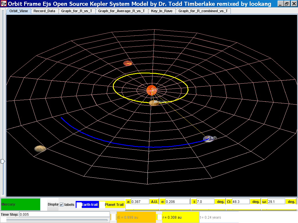
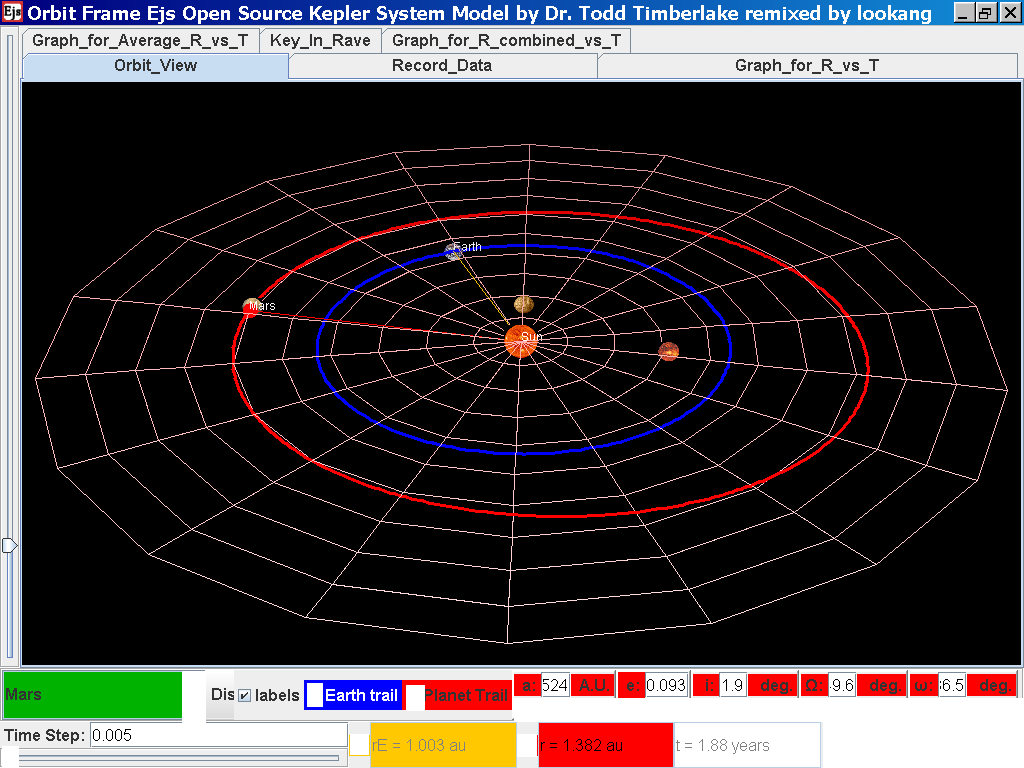
Select from
the drop-down menu the planet, say Mercury to show the orbital
radius and click play.
Click Pause
the simulation when the planet Mercury is almost at the time of 1
complete cycle or period T.
Click Step to
fine tune your determination of period T, say t =0.24 years
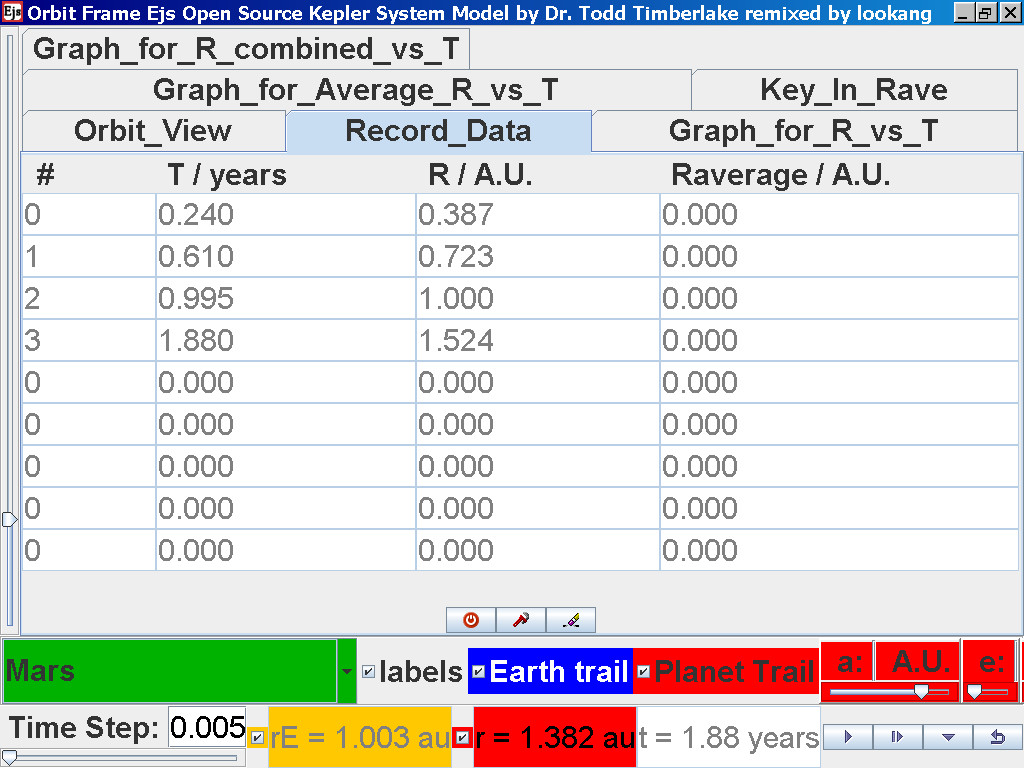
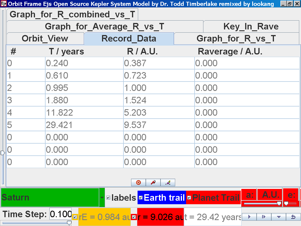
Click on the
adjacent tab Record_Data and select Record Data button to store
this data on the mean radius Rm and period (time for one complete
cycle) T of motion.
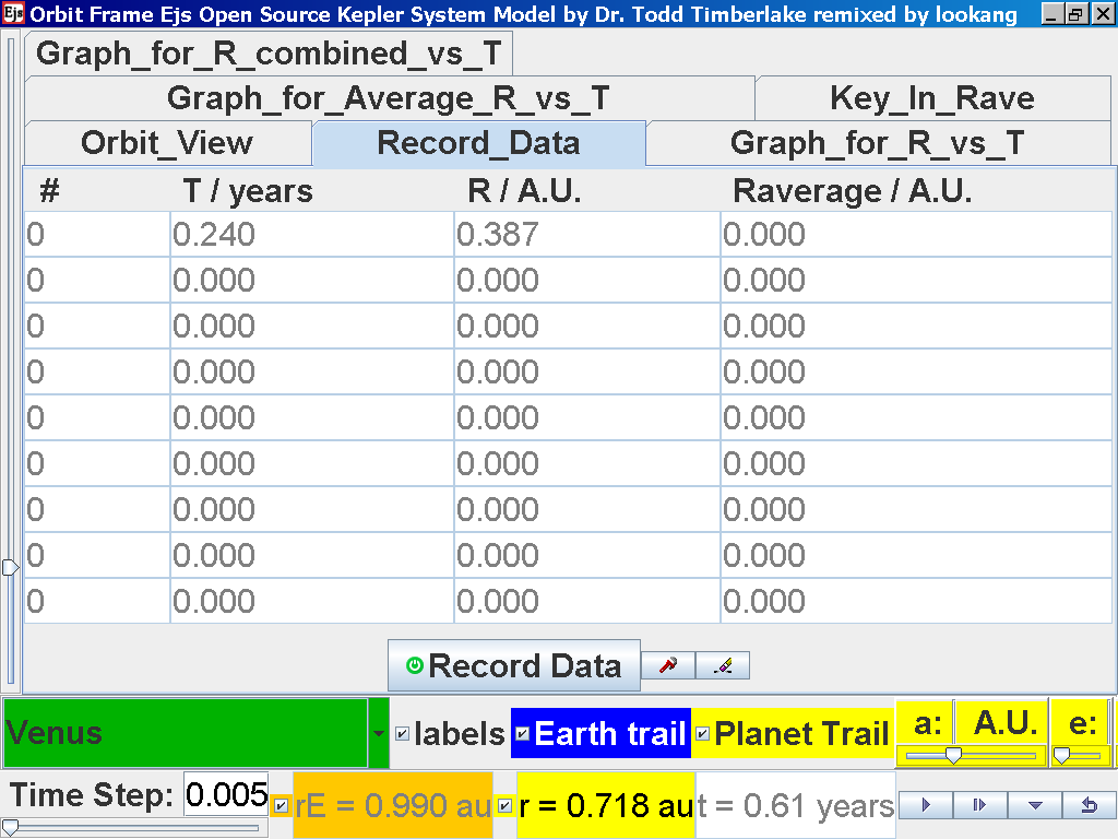
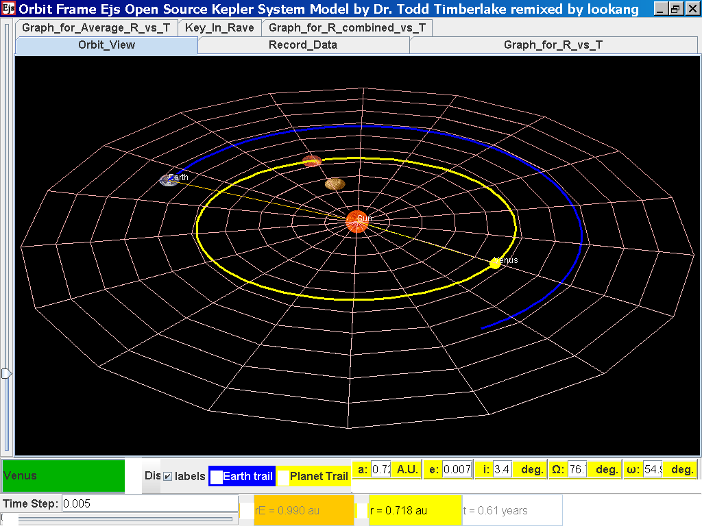
Click back to the Orbit_View and to go
to the next planet to collect data, select from the drop down menu
again and select the next planet say Venus. Play the simulation
for one complete cycle.
again click on the next tab Record_Data
and select Record_Data.
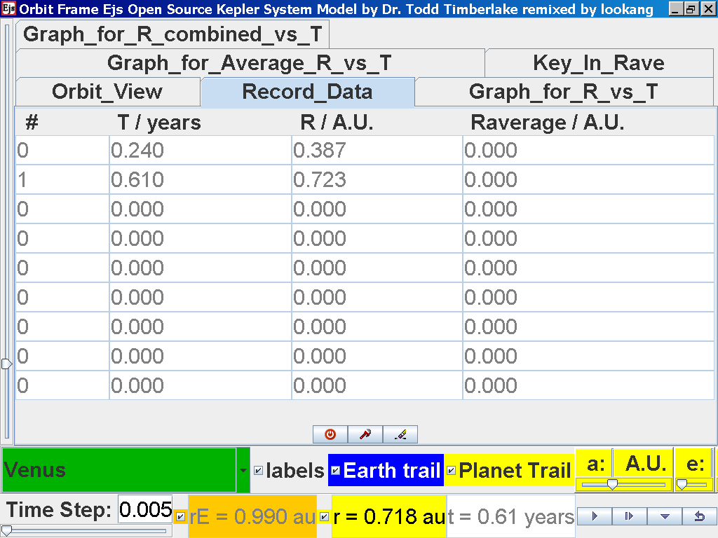
Now the steps need to be repeated for
the rest of the planets. Click back to the Orbit_View and to go to
the next planet to collect data, select from the drop down menu
again and select the next planet say Earth. Play the simulation
for one complete cycle.

again click on the next tab Record_Data
and select Record_Data.

Click back to the Orbit_View and to go
to the next planet to collect data, select from the drop down menu
again and select the next planet say Mars. Play the simulation for
one complete cycle
again click on the next tab Record_Data
and select Record_Data.
Click back to the Orbit_View and to go
to the next planet to collect data, select from the drop down menu
again and select the next planet say Jupiter. Play the simulation
for one complete cycle and increase the time step = 0.08
years reduces the time needed to wait for one cycle.
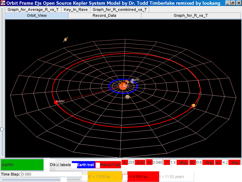
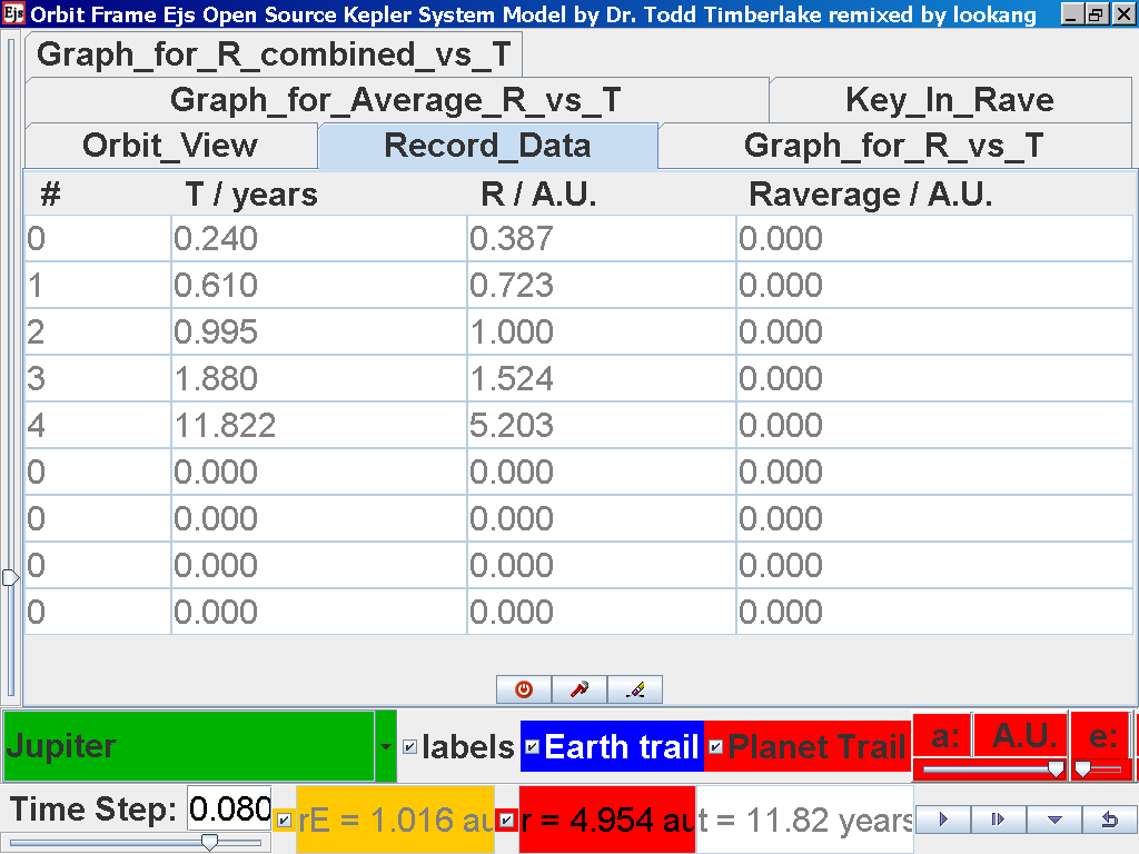
again click on the next tab Record_Data
and select Record_Data.
Click back to the Orbit_View and to go
to the next planet to collect data, select from the drop down menu
again and select the next planet say Saturn. Play the simulation
for one complete cycle
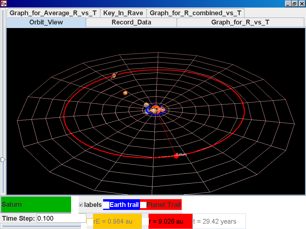
again click on the next tab Record_Data
and select Record_Data.
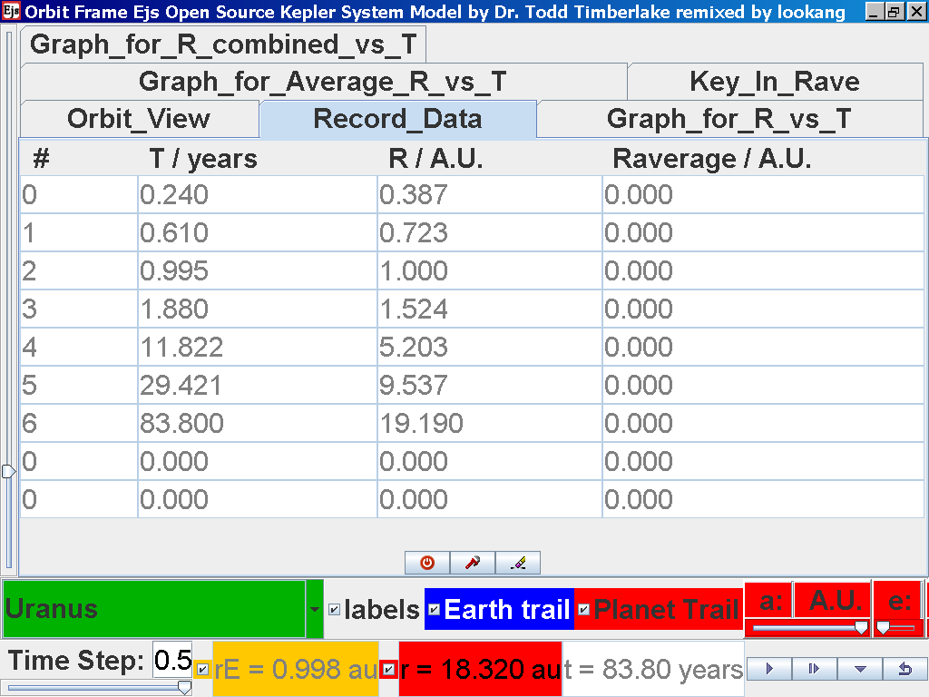
Click back to the Orbit_View and to go
to the next planet to collect data, select from the drop down menu
again and select the next planet say Uranus. Play the simulation
for one complete cycle

again click on the next tab Record_Data
and select Record_Data.
Click back to the Orbit_View and to go
to the next planet to collect data, select from the drop down menu
again and select the next planet say Neptune. Play the simulation
for one complete cycle

again click on the next tab Record_Data
and select Record_Data.

Click back to the Orbit_View and to go
to the next planet to collect data, select from the drop down menu
again and select the next planet say Pluto. Play the simulation
for one complete cycle
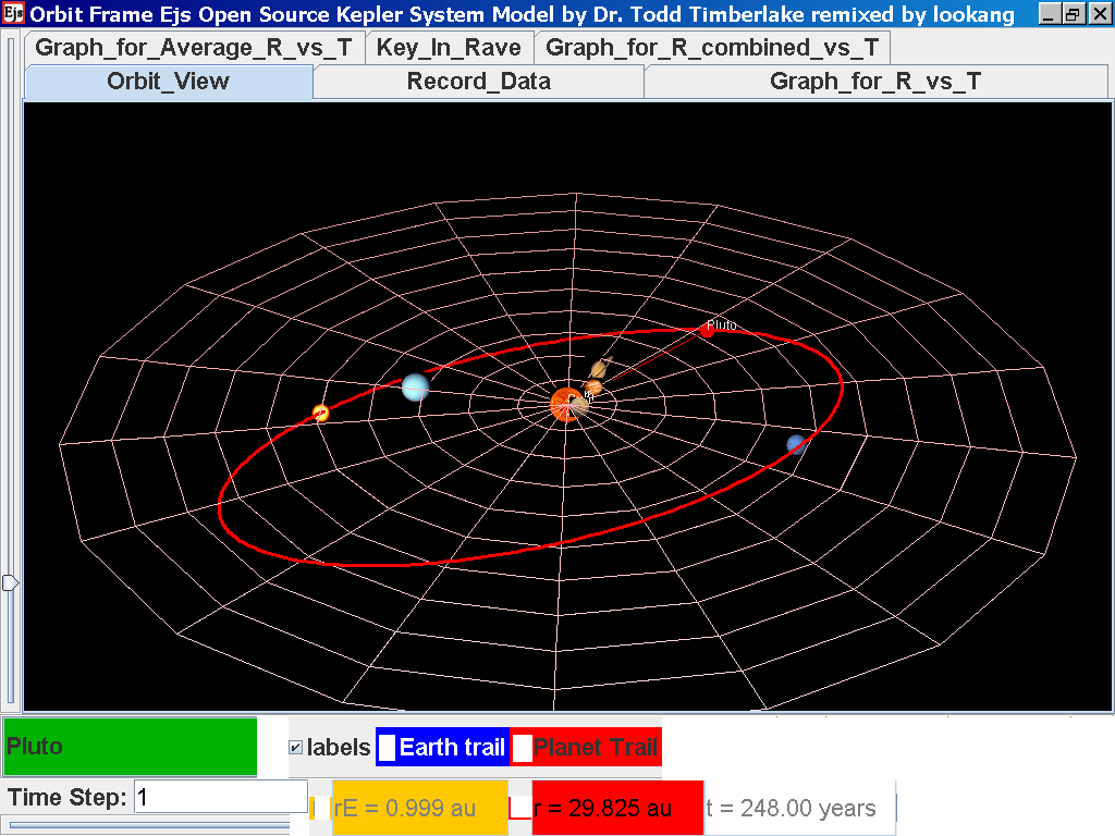
again click on the next tab Record_Data
and select Record_Data.

Notice all the data on the actual T
/years recorded by you is slightly different and the mean radius
of orbits R / A.U. astronomical units which 1 A.U. = mean distance
of Earth to Sun.
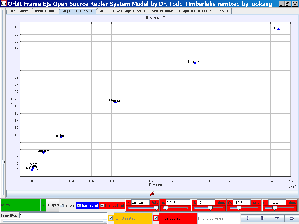
Select the tab Graph_for_R_vs_T and the
simulation automatically plots the data.
Click on the Data Analysis Tool to bring
up the following pop up view for further trend fitting.
Select the Data Builder Button at the
top right corner
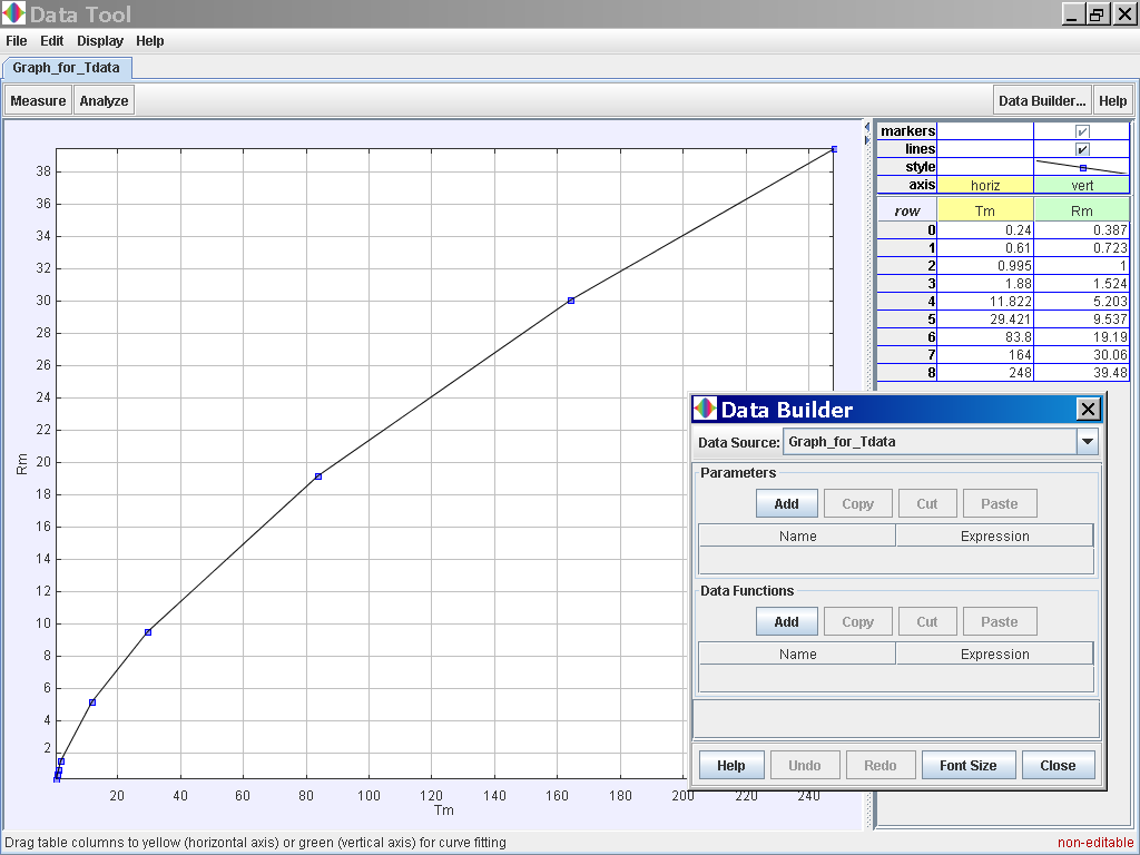
Click on the Data Function Add button to
add your own functions such as T2 for Tmean2 and r3 for
rmean3.
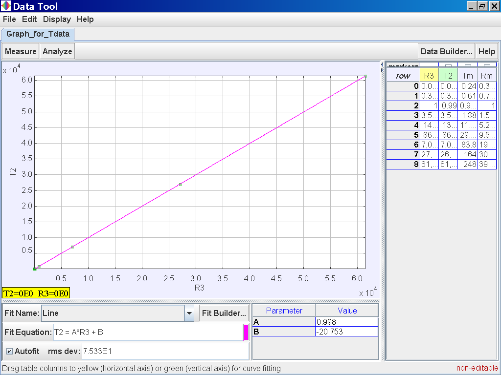
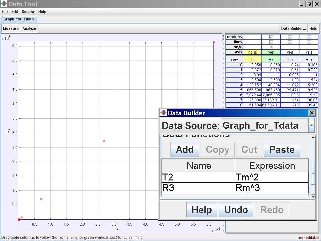 Click on the Analyse button on the top
left corner and select the Linear Fit option of which the data of
T2 and R3 is related
by the following line fit
Click on the Analyse button on the top
left corner and select the Linear Fit option of which the data of
T2 and R3 is related
by the following line fit
T2 =
0.998 R3 -20.753
which suggests T2 α
r3
Alternative activity, you can also
try to log (T) versus log (R)
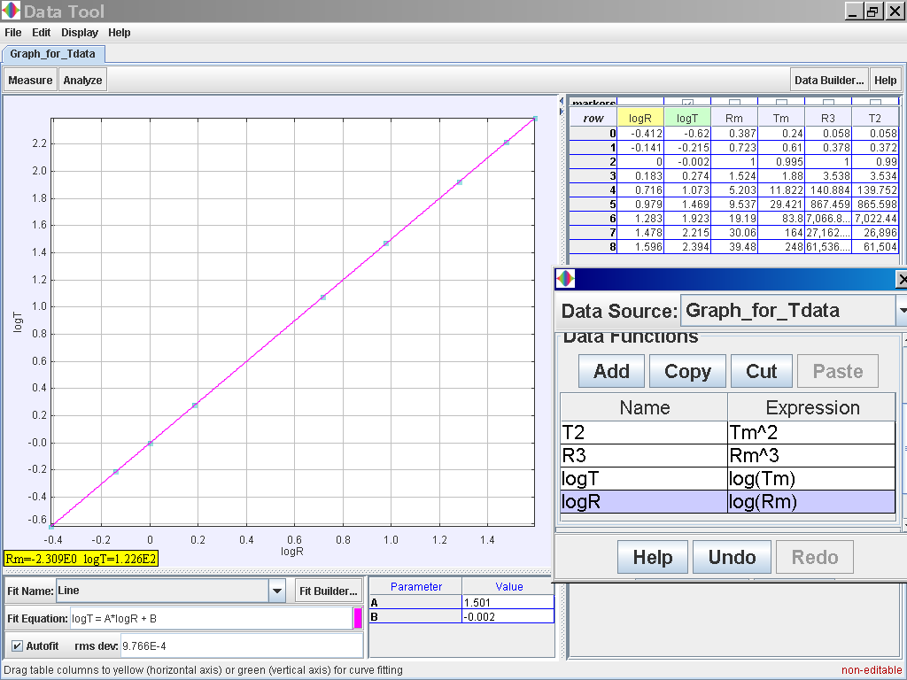 notice again log (T) = 1.501 log (R)
-0.002 which suggests the same relationship of T α r1.5 or simply
T2 α r3
notice again log (T) = 1.501 log (R)
-0.002 which suggests the same relationship of T α r1.5 or simply
T2 α r3
Youtube
https://youtu.be/jt88koyZQuw
Java
Model
http://iwant2study.org/lookangejss/02_newtonianmechanics_7gravity/ejs/ejs_model_KeplerSystem3rdLaw09.jar