Riemann integral

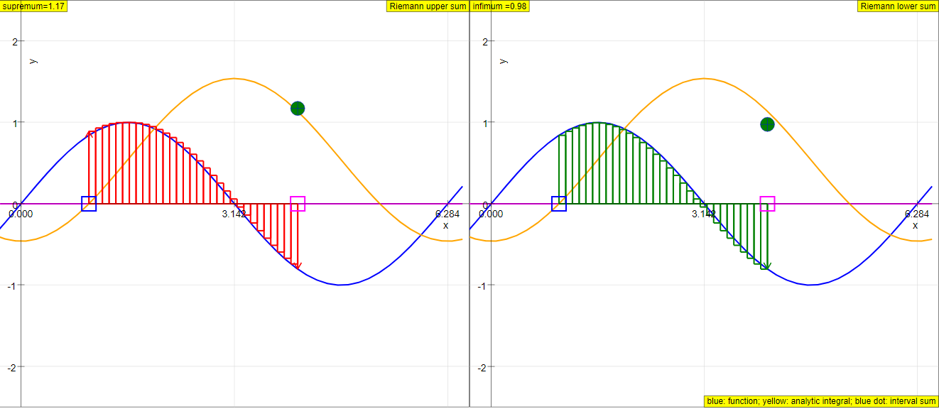
In two dimensions the Rieman integral determines the area between the x axis and the function y = f(x) in an interval x₁ < x < x₂ by nesting it between two approximative sums. Both are constructed by a series of rectangles with intervals along the x axis. For the upper sum the approximative value of y in each interval is equal to the largest value in the interval (its supremum); for the lower sum it is equal to the smalles value (infimum). The Riemann integral exists, when both sums converge with decreasing interval width, and when they converge to the same limit.

The definition is not identical to the classical rectangle algorithm, where the value of the function is equal to the value at the beginning of the interval (more generally: always at the same point in the interval). For "well behaved" functions there will be no difference in results, yet the Riemann definition is more generally applicable.

The approximative calculation of the Riemann integral is shown for the example of a sine function (blue). Its definite integral is to be calculated in the range x₂ - x₁. The initial value x₁ is defined by a slider, the end point x₂ by drawing the red point with the mouse. The yellow curve is the analytic solution cos x - cos x₁.

The number of intervals (n - 1) is defined by slider n. Reset defines 1 < x < 4 and n = 10 (9 intervals) .

The left window shows in red the approximation by the supremum series, with the blue point as the sum; the function always lies below the rectangle. The right window shows the approximation by the infimum series; the function always lies above the rectangle.

Correspondingly the upper sum of the rectangles is always higher than the analytic integral, while the lower sum is always lower - for finite interval widths. With decreasing interval widths both converge to the same value, the Riemann integral.

Experiments

E1: Start with the default setting: x₁ = 1; x₂ = 4; n = 10.

Verify that both graphs really limit the intervals in the y direction by the highest, respectively the lowest value in the interval (observe the sign of the function itself!). Consider the systematic deviation of the sum from the analytic solution.

E2: Compare the construction with the classical rectangle (step) algorithm.

E4: Increase n and observe the process of convergence to the limit value as the interval width decreases.

E4: Draw the end point at a large number for n and observe how the intervals limit lines "paint" the area under the curve. You will not visibly recognize a difference between sum and integral.

E5: Change the initial point with the slider. Draw the end point beyond the initial point and control if the result is still correct.

Translations

Code	Language		Translator	Run

Software Requirements

SoftwareRequirements

	Android	iOS	Windows	MacOS
with best with	Chrome	Chrome	Chrome	Chrome
support full-screen?	Yes. Chrome/Opera No. Firefox/ Samsung Internet	Not yet	Yes	Yes
cannot work on	some mobile browser that don't understand JavaScript such as.....		cannot work on Internet Explorer 9 and below