Exercise by lookang 

Introduction www.bk.psu.edu/faculty/gamberg/mag_lab.doc
A current-carrying wire in a magnetic field experiences a force. The magnitude and direction of this force F, depend on four variables: 
the magnitude and direction of the current (I), 
the strength and direction of the magnetic field (B)
the length of the wire expose to magnetic field is (L)
the angle between the current I and field B is (ϑ) 
Advanced: The force can be described mathematically by the vector cross-product:
O level: Fleming’s Left Hand Rule predicts the using the left hand, F (thumb) B (index finger) I (middle finger)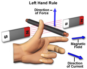 
image from National High Magnetic Field Laboratoryhttp://www.magnet.fsu.edu/education/tutorials/java/handrules/index.html

Advanced: F = I ^ B. L where ^ is the cross product 
O level and A level: F = I . B. L.sin ϑ where ϑ is the angle between I and B 

where
Force F is in newtons N
current I is in amperes A
length L in meters m
magnetic field B in teslas T

The direction of the force F is perpendicular to both the current I and the magnetic field B, and is predicted by the Advanced: right-hand cross-product rule. 
O level and A level: Fleming’s Left Hand Rule

Engage:
a real live demo is the best.!!
a youtube video http://www.youtube.com/watch?v=_X8jKqZVwoI&feature=player_embedded
Engage 1: Would you believe that a wire can jump up even though it is not alive?
Engage 2: have you thought about how a direct current can cause a rotating motion which can be used to drive some simple toys (e.g Tamiya cars) ? 
http://www.tamiya.com/english/products/42183trf502x/top.jpg


Explore
1. Explore the simulation, this simulation is designed with a wire supported by a spring in a system of magnetic fields in y direction.
2 The play button runs the simulation, click it again to pause and the reset button brings the simulation back to its original state.
3 by default values B, I, L, play the simulation. Notice that the wire is in its motionless in its previous state of motion. What is the physics principle simulatted here.
hint: newton's 1st law
4 reset the simulation.
5 using the default values(L = 1 m, ϑ = 90 deg), adjust the value of By =1 and Ix =1 play the simulation. what did you observe? explain the motion in terms of the influences of magnetic field (assume gravitational effect can be neglected, in this computer model gravity is not model)
6 explore the slider z. what do this slider control?
7 explore the slider vz. what does this slider control?
8 by leaving the cursor on the slider, tips will appear to give a description of the slider. you can try it the following sliders such as the drag coefficient b.
9 there are some value of time of simulation t and the checkbox graph for height vs time. 
10 vary the simulation and get a sense of what it does.

11 reset the simulation
Mechanics
12 using the default values (By =0, Ix=0) set z = -0.6, vz=0, b=0). Observe the motion of the wire in the absence of magnetic field. Predict what you will see. Describe the motion of the wire. Explain why this it is so?
hint: select the checkbox to view the scientific graph of height vs t.
13 using the default values (By =0, Ix=0) set z = -0.6, vz=0, b=1). Observe the motion of the wire in the absence of magnetic field. Predict what you will see. Describe the motion of the wire. Explain why this it is so?
hint: select the checkbox to view the scientific graph of height vs t.
14 using the default values (By =0, Ix=0) set z = -0.6, vz=1, b=0). Observe the motion of the wire in the absence of magnetic field. Predict what you will see. Describe the motion of the wire. Explain why this it is so?
hint: select the checkbox to view the scientific graph of height vs t.
15 using the default values (By =0, Ix=0) set z = -0.6, vz=1, b=1). Observe the motion of the wire in the absence of magnetic field. Predict what you will see. Describe the motion of the wire. Explain why this it is so?
hint: select the checkbox to view the scientific graph of height vs t.
16 conduct more scientific inquiry into the simulation if need before the next part of the question.
Elaborate 
17 explain the effects of b, the model used is drag force = b.v.

18 reset the simulation
Magnetic Force
Evaluate:
19 A scientist hypothesis "O level and A level: F = I . B. L. where ϑ =90 deg" play the simulation for different initial condition and design an experiment with tables of values to record systematically, determine whether the hypothesis is accurate. 

20 what is the impact of the ϑ != 90 deg ?
21 Suggest a better hypothesis
22 This computer model does not build in gravity, suggest with reason(s) why you agree or disagree with this statement. You can examine and modify this compiled EJS model if you run the model (double click on the model's jar file), right-click within a plot, and select "Open EJS Model" from the pop-up menu.  You must, of course, have EJS installed on your computer.  Information about EJS is available at: and in the OSP comPADRE collection 


Have Fun!