About

Description

Description of the simulation window

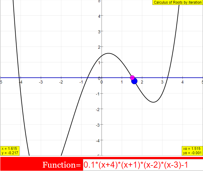
The simulation has two windows with an x, y coordinate system. As default the left one shows a power function (parabola) of fourth grade. Its roots are to be calculated (the x values for which y is zero). Its formula is visible in a text field:

y = 0.1(x+4)(x+1)(x-2)(x-3)-0.1

= 0.1(x⁴ - 3x² + 10x + 23)

The first formulation indicates that there are 4 roots which are near to the integers -4, -1, 2 and 3. Substituting the constant element (-0.1) by 0, these integers would be exact solutions. The roots of the predefined function are irrational numbers.

The range of the x coordinate goes from -x_max to +x_max. The default value of x_max is 5; it can be changed in the number field. The range of the y coordinate goes from -12 to +12. Changing to another y scaling is achieved by using appropriate factors (default 0,1) in the editable formula.

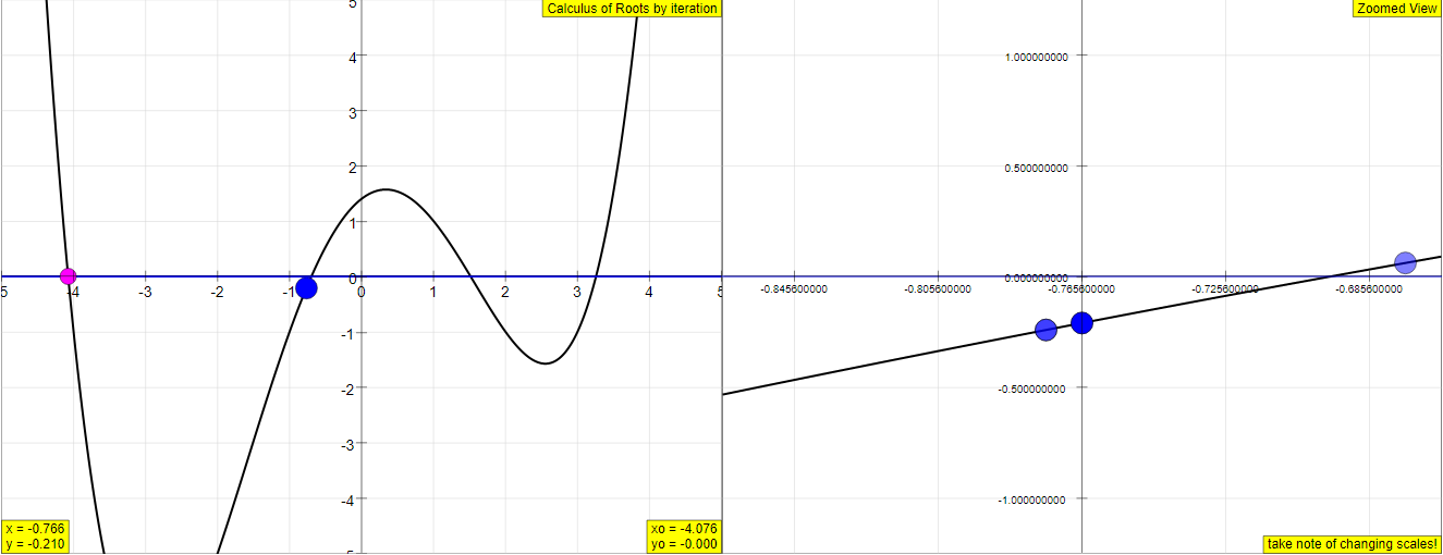
The magenta colored point is the starting point of the calculation (default x₀= - 4.5). It can be drawn with the mouse along the function curve to another abscissa. While the blue iteration points wanders along the curve in the positive x direction, the starting point stays fixed till a root has been calculated with the required accuracy delta. Then it will jump to this root.

The required deviation from exactly zero delta = y -0 can be defined in the white number field (default 0.00001). The current deviation during the calculation process is shown in the gray y field below. Two gray number fields retain the values xo and y0 of the initial point and hence also of the last root found.

The current iteration point is shown in blue. Once a root has been calculated with the required precision, it jumps to the first point of the next iteration.

At high accuracy, the movement of the iteration point will no longer be recognizable after a few iteration steps. For this reason the right window shows a zoomed section of the curve with self adjusting scales. Up o 4 consecutive points of the iteration are retained, the current one blue, three trailing ones in red (after a flyback blue and red coincide for one point).

In the zoom window one can follow the flybacks of the iteration process and the reduction of the x step by a factor of 10 at such an event up to the highest resolution. During this process the curve will appear more and more like a straight line.

The Start/ Stop button controls the iteration process. Restart leads back to the default situation. The number of iteration steps per second is defined by the slider speed between 1 and 25 (default 2). Default stops the iteration when a root has been found; to get the next one shift the initial point with the mouse and Start again. Refusing the Option One root only calculates all roots in consecutve order.

The speed of the Simulation is determined by the stepwise time control of visualization. It has no relation to the very short time interval which the computer would need to calculate a new root without these interruptions

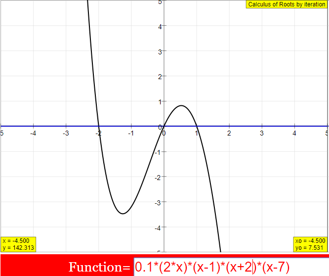
The text field of the formula is editable. You can input any formula to determine its roots. Take care to adjust x_max and the ordinate scale to the specifics of the function.

Iteration Algorithm

Iteration algorithm

The equation f(x) = g(x)

can be formulated as f(x) - g(x) = 0

Hence the general task to determine conditions of equality of 2 functions for a value x is reduced to finding the roots of one equation, where its value is zero. If g(x) is a number q, the task is to find a value x for which f(x) has the value q.

Logically the task presents the inversion of the simple task to calculate the value of f(x) for a given x. Yet an analytic solution is possible only for very simple functions, as a linear or a second order parabola. With trigonometric functions or logarithms, in classical technique, we use tables of corresponding numbers, without normally asking how they originated.

Numerically the roots of any function can be calculated by iteration up to every wanted, finite degree of accuracy. Instead of looking for an inverting calculus, we simply calculate "forward". We take an initial arbitrary value of x and calculate y = f(x). In general y will not be zero, and hence x will not be a root. Now we vary x systematically (iterate x) until y becomes smaller than a desired accuracy delta.

For easy understanding and demonstration this simulation uses a very simple iteration algorithm in form of a calculating loop. In each step of the loop the following commands are performed (you will find the code at the Evolution page of the EJS model);

d x = 0.1/n; defines the step width in dependence on a step variable n

x = x + dx; goes one step further

the corresponding y- value is calculated with the given formula for f(x) (Fixed Relations page)

if (y>0) ( it is assumed that initially y<0, with changing sign (y>0) a root has been crossed) {

x = x - 2*dx; jump back to last point

n=10*n; reduce step by factor 10

}

if (Math.abs(y)<2*delta) when y is sufficiently small {

_pause(); -stop calculation

}

While this algorithm is very simple and easy to understand, it needs many steps. One can speed it up considerably using variable step widths, that adjust themselves to the steepness of the curve or even to its curvature. In the zoom window one recognizes that the function can quickly be approximated well by a linear. The root of a linear determined by 2 consecutive points of the iteration or even of a parabola determined by 3 of them, will be very close to the root of the curve itself after just one more step of iteration. The linear approximation is used in the so called Newton algorithm.

With the availability of fast PCs the time needed for iteration algorithms is so minute that one can use them universally. Standard programs like Excel or Mathematica offer ready solutions.

Our simple algorithm is easily extended to calculate all roots in a given interval in one run. An additional if- else- logic condition is sufficient to adjust the flyback command to the 2 cases of the initial y value being positive or negative.

if (y0<0) {

dx = 0.1/n;

x = x + dx;

if (y > 0) {

x = x - 2*dx;

n = 10*n;

}}

else {

dx = 0.1/n;

x = x + dx;

if (y < 0) {

x = x - 2*dx;

n =10*n;

}}

As the formula field is editable, one can determine roots for any arbitrary function.

Experiments

E1: Start the default situation. Watch the flybacks with changing step width in the zoom window, and the changes in the number fields.

E2: After Reset increase speed to 10. In the zoom window the consecution of the iteration point, the formation of the trailing followers and the jump back after crossing a root will be better recognizable.

E4: Change speed to 1. Stop iteration after a flyback. Using the Start/Stop button you can now follow single steps. In the zoom window you can follow the jumps in scaling of both abcissa and ordinate.

E5: Change speed while the iteration runs.

E6: Change the residual value delta over a wide range and control if it is really achieved.

E7: Draw the initial point and calculate the 4 roots separately this way.

E8: Delete the constant element in the formula window. Now the roots should be integers. Control the achieved accuracy!

E9: Change the formula in the formula field to 10*sin(x) (factor 10 for adjustment to the y scale). Calculate the first root. Repeat the calculation for different values of delta. Compare the results to π = 3.14159 26535 89793...

E10: Calculate roots for functions of your own.

Translations

Code	Language		Translator	Run

Software Requirements

SoftwareRequirements

	Android	iOS	Windows	MacOS
with best with	Chrome	Chrome	Chrome	Chrome
support full-screen?	Yes. Chrome/Opera No. Firefox/ Samsung Internet	Not yet	Yes	Yes
cannot work on	some mobile browser that don't understand JavaScript such as.....		cannot work on Internet Explorer 9 and below