


About
Two-body Newtonian Gravitation
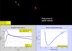
Simulation of Newtonian gravitation for a two-body system. The simulation panel is a visualisation of the motion of the two bodies, the larger one (red) of variable mass M and the smaller one (blue) of fixed mass m. There are three (plus one) graphs:
- Radial and tangential velocities of the smaller mass m as functions of time. Cartesian components can also be shown.
- Potential, kinetic, and total energy as functions of time for the system.
- Visualisation of the analytic expressions of energy as a function of radial separation (the effective one-body system). This consists of two graphs: (i) a dynamic visualisation that tracks the system evolution and motion, as well as (ii) a static visualisation in a separate graph showing the analytic expression as a sum of gravitational and "centrifugal (associated with angular momentum)" terms. The graphs are separated because of the different vertical scales needed for each visualisation.
Instructions
- The slider allows you to vary the ratio of masses M/m.
- You can also vary the initial velocity of the smaller mass m in various ways: (i) click and drag the head of the velocity arrow; (ii) input values individually for the components (vx, vy); (iii) click the checkbox to autocalculate initial velocity for a circular orbit.
- Click play/pause/reset. You can readjust parameters while the simulation is paused. The graphs will be refreshed.
Interpreting the Graphs
In the velocity-time graph, the blue/black lines are the radial/tangential velocities of the smaller (blue) mass m. These are calculated as the simulation is running. Cartesian components of the velocity can also be shown as dashed lines.
In the energy-time graph, the red line is the kinetic energy of the larger (red) mass M, while the blue line is the kinetic energy of the smaller (blue) mass m. The black line is the gravitational potential energy of their interaction, while the dashed line is the total energy (if shown). These are calculated as the simulation is running.
In the energy-position graphs, the analytic form for the effective radial potential energy is shown, as a function of the radial separation between the two masses, which is based on analysing the relative motion as a one-body problem. Exact expressions are used for the angular momentum of the system, which provides a "centrifugal" term to the effective radial potential energy. The total energy is shown as a dashed line. In the dynamic visualisation, the radial potential energy is calculated and traced when the simulation is running. In the static visualisation, the vertical scale is larger to show how U_{eff} = GPE + L^2 term. The orbital eccentricity is also displayed as a text overlay.
Notes
The simulation automatically sets the initial conditions (position, velocity) for the larger (red) mass such that the centre of mass (white) is stationary at the centre of the simulation panel.
Translations
| Code | Language | Translator | Run | |
|---|---|---|---|---|
 |
||||
Software Requirements
| Android | iOS | Windows | MacOS | |
| with best with | Chrome | Chrome | Chrome | Chrome |
| support full-screen? | Yes. Chrome/Opera No. Firefox/ Samsung Internet | Not yet | Yes | Yes |
| cannot work on | some mobile browser that don't understand JavaScript such as..... | cannot work on Internet Explorer 9 and below |
Credits
 Zhiming Darren TAN
end faq
Sample Learning Goals
[text]
For Teachers
[text]
Research
[text]
Video
[text]
Version:
Other Resources
[text]
