


About
The logistic map
The logistic equation was first proposed by Robert May as a simple model of population dynamics. This equation can be written as a one-dimensional difference equation that transforms the population in one generation, xn, into a succeeding generation, xn+1.
xn+1 = 4 r xn (1-xn)
Because the population is scaled so that the maximum value is one, the domain of x falls on the interval [0; 1].
The behavior of the logistic equation depends on the value of the growth parameter, r. If the growth parameter is less than a critical value r<0.75..., then x approaches a stable fixed value. Above this value for r, the behavior of x begins to change. First the population begins to oscillate between two values. If r increases further, then x oscillates between four values, then eight values. This doubling ends when r > 0.8924864... after which almost any x value is possible.
Generalized logistic map
xn+1 = 4rxn(1-xn) = 4 r ( xn -xn2)
The logistic series rule sets the next generation proportional to the existing one in its first term. This alone would lead to exponential growth for r > 1/4, and to exponential decline for r < 1/4). The second term introduces a diminution that depends on the square of the existing population (note that in the above formulation xn < 1 , hence xn2 < xn ).
The issue for a given growth rate r is: will the population approach a stable equilibrium (limit) value of linear growth and quadratic extinction − assuming an unlimited number of generations under identical conditions. If so, how does the equilibrium value depend on the growth rate r ?
Growth exists when xn+1 > xn, hence r > 1/(4(1-xn)). As 0 < x < 1 , for r < 0.25, all populations will iterate to zero, independent of the starting value. If for r > 0.25 an equilibrium value exists, a starting population greater than the limit should shrink to it, smaller ones should expand to it.
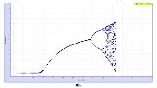
In the simulation r is increased in steps of 0.001 in the range 0 < r < 1 . The calculation for each step starts with a random value 0 < x1< 1 . In a calculation loop 2000 members of the series are calculated. The first ones differ largely in dependence on the random initial value. Therefore the first 1000 iterations are suppressed in the chart. For each step in r 1000 points on the ordinate could represent the iterations 1000 to 2000.
In the range 0.25 < r < 0.75 the iterations are so close together that they appear as one point only, resulting in a "limit curve" in dependence on r.
Then the curve splits in two (bifurcation), which means that the iteration now has two accumulation points for a certain r. The bifurcation repeats itself, until no accumulation points are visible any longer.
Quite surprisingly between the "filled" bands there are some quasi "empty" bands with only a few accumulation points.
The determining term is the product 4r; factors different from 4 just scale the abscissa differently.
It is not decisive for the bifurcation that the limiting term is exactly (1-xn). The crucial point is the nonlinearity of the conjunction xn -xn2.
To demonstrate this, a generalized series rule is used in this simulation, using a term (1-xnk), with k > 0 :
xn+1 = 4rxn(1-xnk)
When opening the simulation k = 1; Start produces the common logistic map.
After Stop k can be changed in the range 0.1 < k < 2 by a slider. The abscissa scaling is adjusted automatically.
The left chart displays the total range, the right one that of bifurcation with higher resolution. One can differentiate the calculation steps and the bifurcation structure in more detail if the window is expanded to full screen size.
Author von LogisticMap.xlm : Francisco Esquembre and Wolfgang Christian.
Text and original idea from the Open Source Physics project manual
Date : July 2003
Generalized by Dieter Roess in August 08
This simulation is part of
“Learning and Teaching Mathematics using Simulations
– Plus 2000 Examples from Physics”
ISBN 978-3-11-025005-3, Walter de Gruyter GmbH & Co. KG
Translations
| Code | Language | Translator | Run | |
|---|---|---|---|---|
 |
||||
Software Requirements
| Android | iOS | Windows | MacOS | |
| with best with | Chrome | Chrome | Chrome | Chrome |
| support full-screen? | Yes. Chrome/Opera No. Firefox/ Samsung Internet | Not yet | Yes | Yes |
| cannot work on | some mobile browser that don't understand JavaScript such as..... | cannot work on Internet Explorer 9 and below |
Credits

![]()
 Dieter Roess - WEH- Foundation; Tan Wei Chiong; Lookang Wee; Wolfgang Christian; Francisco Esquembre
end faq
For Teachers
The Logistic Map is used to model population growth using the following equation: x(n+1) = rx(n)(1 - x(n))
Where x represents the ratio of the existing population to the maximum possible population, n represents the number of iterations, and r is a parameter ranging between 0 and 4 that changes the behaviour of the population growth.
In this simulation, we denote the parameter r by 4r, where r now ranges between 0 and 1. From here on, when we refer to r, we mean the r in the simulation that ranges between 0 and 1.
This model simulates the effects of reproduction, where the population size increases at a rate proportional to the current population when the population is small, and starvation, where the population size decreases at a rate proportional to the carrying capacity of the environment.
It is not decisive for the bifurcation that the limiting term is exactly (1-x(n)). The crucial point is the non-linearity of the conjunction x(n) -x(n)^2.
To demonstrate this, a generalized series rule is used in this simulation, using a term (1-x(n)^k), with k > 0 :
x(n+1) = 4rx(n)(1-x(n)^k)
When r is approximately 0.89 to 1, the population size starts to exhibit chaotic behaviour, fluctuating wildly between many values. In fact, the Logistic Map is commonly used to show how chaotic systems can arise from seemingly simple models.
Author : Francisco Esquembre and Wolfgang Christian, JavaScript version Wei Chiong and Loo Kang
Text and original idea from the Open Source Physics project manual
Date : July 2003 and JavaScript 2018
Video
[text]
Version:
- http://phy01.phy.ntnu.edu.tw/ntnujava/index.php?topic=1817.0
- https://weelookang.blogspot.com/2018/05/logistic-map-javascript-simulation.html
Other Resources
[text]
