


About
Fourier coefficients
The Fourier series of a periodic function f(x) with period x = 2π is of the form
f(x) = a0 /2 + Σ (ancos(nx) + bnsin(nx)); n=1,2,3....∞
To calculate the coefficients of the series, one starts with the following assumed identities:
∫f(x)cos(mx)dx = ∫cos(mx) Σ(a0/2 + Σ ancos(nx) + bnsin(nx))dx
∫f(x)sin(mx)dx = ∫sin(mx) Σ(a0/2 + Σ ancos(nx) + bnsin(nx))dx
where one integrates over one base period (m = 1).
Suppressing constants, the following types of integral are to be evaluated, summed over index n:
With m = 1,2,3...∞ and n = 1,2,3...∞: order of the harmonic (fundamental m, n = 1)
cos (mx)
sin (mx)
cos (mx) * (a*cos (nx) + b*sin (nx))
sin (mx) * (a*cos (nx) + b*sin(nx))
All integrals are zero except of those few where the indices are identical: m = n and the function types are the same (sine or cosine). Therefore every sum for a specific index n has only one member and the coefficients can easily be derived from the reduced equations as:
a0 = 2/T∫f(t) dt
an= 2/T∫cos(nx) f(t) dt
bn = 2/T∫sin(nx) f(t) dt
This simulation demonstrates the different types of functions and their integral.
Operation of the simulation
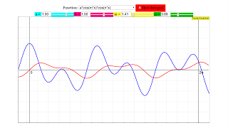
A ComboBox holds a list of all function combinations described on the Fourier Coefficients page. When one is selected it is displayed in red. The antiderivative is calculated for the fundamental period and drawn as a blue curve. Its end value at x = 2pi is the definite integral over one fundamental period, which is needed for the calculation of the coefficients. The integration process is slowed down to visualize more clearly the consequence of changes in parameters or indices.
Some of the selectable functions contain parameters a and b which can be changed continuously by sliders a/ b . Two other sliders m/n select the critical indices m and n as real numbers between 1 and 10.
Parameters and indices are maintained when functions are changed. Integration is started automatically at any change as long as the selection Integral remains active.
By means of sliders a and b scaling of the ordinate can be adjusted to the specific function. They also allow phase shifting of functions.
E1: Choose cosx in the comboBox. It will be calculated and displayed in red. Activate the Integral check box. The integration process will begin with the initial value of the function at x = 0 and will progress in red to the end of the fundamental period x = 2 π. Reflect why the end value and hence the definite integral over the interval [0, 2pi] is zero for integer n.
E2: Change index n with the slider and watch the integral curve. Reflect again why the definite integral is always zero for integer n.
E3: Choose sinx and verify the experiments for it.
E4: Choose asinx + bcosnx and assure yourself by varying a, b, n that the superposition is always a simple, phase shifted periodical, whose definite integral is zero for integer n.
E5: Choose cosx * sinx and assure yourself that the definite integral is always zero for integer n.
E6: Choose the remaining "mixed" functions and assure yourself that the definite integral is non zero only when both terms are of the same type and have identical indices.
E7: Integrate some of the functions analytically and verify the experimental findings.
E8: Conclude in general which characteristics of the functions sine and cosine are the base of your results.
This file was created by Dieter Roess November 2008
This simulation is part of
“Learning and Teaching Mathematics using Simulations
– Plus 2000 Examples from Physics”
ISBN 978-3-11-025005-3, Walter de Gruyter GmbH & Co. KG
Translations
| Code | Language | Translator | Run | |
|---|---|---|---|---|
 |
||||
Software Requirements
| Android | iOS | Windows | MacOS | |
| with best with | Chrome | Chrome | Chrome | Chrome |
| support full-screen? | Yes. Chrome/Opera No. Firefox/ Samsung Internet | Not yet | Yes | Yes |
| cannot work on | some mobile browser that don't understand JavaScript such as..... | cannot work on Internet Explorer 9 and below |
Credits
 Dieter Roess - WEH- Foundation; Tan Wei Chiong; Loo Kang Wee
end faq
Sample Learning Goals
[text]
For Teachers
The Fourier Series is a series that decomposes any periodic curves into a sum of sines and cosines.
In this simulation, you are instead given several functions with multiple parameters a, b, m, n to select from and you can adjust them with either the sliders or the fields provided. The appearance of the periodic wave will change accordingly.
There is also a red checkbox labeled "Show Integral" that when checked, does exactly what it says.
The integral is shown in red, and the value of the integral curve at a point denotes the net area under the curve from 0 to that point. Do play around with the parameters and see how it affects the curve.
Research
[text]
Video
[text]
Version:
- http://weelookang.blogspot.sg/2016/02/vector-addition-b-c-model-with.html improved version with joseph chua's inputs
- http://weelookang.blogspot.sg/2014/10/vector-addition-model.html original simulation by lookang
Other Resources
[text]