🚤PICUP Harmonic and Anharmonic Oscillations of a Boat JavaScript Simulation Applet HTML5

Breadcrumbs

http://iwant2study.org/lookangejss/02_newtonianmechanics_8oscillations/ejss_model_PICUP_vhull_frem_v2/

About

intro

Harmonic and Anharmonic Oscillations of a Boat

Developed by E. Ayars

Easy JavaScript Simulation by Fremont Teng and Loo Kang Wee

Simple Harmonic Oscillation (SHO) is everyone’s favorite type of periodic motion. It’s simple, easy to understand, and has a known solution. But SHO is not the only kind of periodic motion. In this set of exercises we’ll investigate an anharmonic oscillator. We’ll explore characteristics of its motion, and try to get an understanding of the circumstances under which the motion can be approximated as simple harmonic.

Subject Area	Mechanics
Levels	First Year and Beyond the First Year
Available Implementations	Python and Mathematica Easy JavaScript Simulation
Learning Objectives	Students who complete these exercises will be able to use an ODE solver to develop a qualitative understanding of the behavior of an anharmonic oscillator. Most students gain a good understanding of the behavior of harmonic oscillators in their introductory classes, but not all oscillators are harmonic. Here we investigate an idealized boat hull which exhibits asymmetric oscillation: the restoring force is stronger for displacements in one direction than in the other. This results, for large oscillations, in a visibly non-sinusoidal oscillation. For small oscillations, the motion is approximately simple harmonic again.
Time to Complete	120 min

instructorguide

This set of exercises guides students through the development of an anharmonic oscillator, then lets them use an ODE solver to plot the motion. It does not describe how to use an ODE solver. Emphasis is on qualitative understanding of the system, although if the instructor chooses it is certainly possible to use real parameters ( $ρ_{w a t e r}$ , dimensions of boat, etc) to obtain an “engineer’s answer”.

The problem is accessible to first-year students, but it may also be of interest to students in higher-level courses.

There is opportunity to discuss limitations of the model on the final problem. In this problem, if the amplitude is high enough that the boat gets out of the water, the model in the ODE breaks down in interesting and spectacular ways.

The pseudocode, Mathematica notebook, python code, and sample solutions of this Exercise Set assume the use of built-in differential equation solving capabilities. Depending on instructor preference, it may be desirable for students to have experienced the direct application of a finite-difference algorithm to a variety of first-order differential equations before using a computational ‘black box.’

theory

The simplest example of Simple Harmonic Oscillation (SHO) is a mass hanging on a spring. In equilibrium, the string will have stretched some equilibrium distance $x_{o}$ , so that the weight of the mass $m g$ is balanced by the spring force $- k x_{o}$ . Any additional motion $x$ of the spring will result in an unbalanced force:

Σ F = m a = m g - k (x o + x) (1)

md2xdt2=(mg−kxo)−kx(2)md2xdt2=(mg−kxo)−kx<math xmlns="http://www.w3.org/1998/Math/MathML" display="block"><mtable displaystyle="true"><mlabeledtr><mtd id="mjx-eqn-2"><mtext>(2)</mtext></mtd><mtd><mi>m</mi><mfrac><mrow><msup><mi>d</mi><mn>2</mn></msup><mi>x</mi></mrow><mrow><mi>d</mi><msup><mi>t</mi><mn>2</mn></msup></mrow></mfrac><mo>=</mo><mo stretchy="false">(</mo><mi>m</mi><mi>g</mi><mo>−</mo><mi>k</mi><msub><mi>x</mi><mi>o</mi></msub><mo stretchy="false">)</mo><mo>−</mo><mi>k</mi><mi>x</mi></mtd></mlabeledtr></mtable></math>

d2xdt2=−kmx(3)d2xdt2=−kmx<math xmlns="http://www.w3.org/1998/Math/MathML" display="block"><mtable displaystyle="true"><mlabeledtr><mtd id="mjx-eqn-3"><mtext>(3)</mtext></mtd><mtd><mfrac><mrow><msup><mi>d</mi><mn>2</mn></msup><mi>x</mi></mrow><mrow><mi>d</mi><msup><mi>t</mi><mn>2</mn></msup></mrow></mfrac><mo>=</mo><mo>−</mo><mfrac><mi>k</mi><mi>m</mi></mfrac><mi>x</mi></mtd></mlabeledtr></mtable></math>

This last equation is in the form of the equation for SHO:

d2xdt2=−ω2x(4)d2xdt2=−ω2x<math xmlns="http://www.w3.org/1998/Math/MathML" display="block"><mtable displaystyle="true"><mlabeledtr><mtd id="mjx-eqn-4"><mtext>(4)</mtext></mtd><mtd><mfrac><mrow><msup><mi>d</mi><mn>2</mn></msup><mi>x</mi></mrow><mrow><mi>d</mi><msup><mi>t</mi><mn>2</mn></msup></mrow></mfrac><mo>=</mo><mo>−</mo><msup><mi>ω</mi><mn>2</mn></msup><mi>x</mi></mtd></mlabeledtr></mtable></math>

where $ω \equiv \sqrt{\frac{k}{m}}$ in this case. Knowing $ω$ , we can then go on to do whatever we need to do with the problem. The period of the motion is $T = \frac{2 π}{ω}$ , the position as a function of time will be $x (t) = A \cos (ω t + ϕ)$ , etc.

We can use this “known solution” to SHO any time we can get the equation of motion into the form of the SHO differential equation. If the second derivative of a variable is equal to a negative constant times the variable, the solution is SHO with $ω$ equal to the square root of that constant.

Even when we can’t get the equation of motion for a system into the form of SHO, we can often approximate the motion as SHO for small oscillations. The classic example of this is the simple pendulum. The equation of motion for the pendulum is

d2θdt2=−gLsinθ(5)d2θdt2=−gLsinθ<math xmlns="http://www.w3.org/1998/Math/MathML" display="block"><mtable displaystyle="true"><mlabeledtr><mtd id="mjx-eqn-5"><mtext>(5)</mtext></mtd><mtd><mfrac><mrow><msup><mi>d</mi><mn>2</mn></msup><mi>θ</mi></mrow><mrow><mi>d</mi><msup><mi>t</mi><mn>2</mn></msup></mrow></mfrac><mo>=</mo><mo>−</mo><mfrac><mi>g</mi><mi>L</mi></mfrac><mi>sin</mi><mo>⁡</mo><mi>θ</mi></mtd></mlabeledtr></mtable></math>

This equation is not SHO, but for small $θ$ , $\sin θ \approx θ$ so we can approximate the motion as SHO as long as the oscillations are small.

In the case of our wedge-shaped boat, the equation of motion is

d2γdt2=−ω2o(1+γ2)γ(6)d2γdt2=−ω2o(1+γ2)γ<math xmlns="http://www.w3.org/1998/Math/MathML" display="block"><mtable displaystyle="true"><mlabeledtr><mtd id="mjx-eqn-6"><mtext>(6)</mtext></mtd><mtd><mfrac><mrow><msup><mi>d</mi><mn>2</mn></msup><mi>γ</mi></mrow><mrow><mi>d</mi><msup><mi>t</mi><mn>2</mn></msup></mrow></mfrac><mo>=</mo><mo>−</mo><msubsup><mi>ω</mi><mi>o</mi><mn>2</mn></msubsup><mrow><mo>(</mo><mrow><mn>1</mn><mo>+</mo><mfrac><mi>γ</mi><mn>2</mn></mfrac></mrow><mo>)</mo></mrow><mi>γ</mi></mtd></mlabeledtr></mtable></math>

This is not SHO! If $γ$ is small, it is approximately SHO, but only approximately.

Note: The Mathematica and Python solutions here make use of built-in tools for solving differential equations. For other implementations the reader is directed to Numerical Recipes in C, or equivalent text, which will provide an introduction and theoretical description of the numerical approach to solutions via finite-difference methods.

exercises

Exercise 1: A straight-sided boat

Imagine a boat with vertical sides, floating. There will be two forces on this boat: its weight $m g$ , and the buoyant force $- ρ g V$ . (I’ve defined down to be the positive direction, here, so the buoyant force is negative since it’s upwards.) The volume $V$ in the buoyant force component is the volume of water displaced by the boat: in other words, the volume of boat that is below water level. In equilibrium, the bottom of the boat will be some distance $x_{o}$ below the water, so $V = A x_{o}$ , where $A$ is the area of the boat at the waterline.

If we then push the boat down some additional distance $x$ and let go, the boat will bob up and down.

Show that the boat’s vertical motion is SHO. It will probably be helpful to follow the same pattern as for the introduction example: the key is to get the equation in the form of the equation for SHO.
What is the period of the boat’s motion?

Exercise 2: A V-hulled boat

Instead of a straight-sided boat, imagine a boat with a V-shaped hull profile, as shown below.

Sketch of a boat with a V-shaped hull

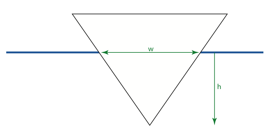
The width $w$ of the hull at the waterline depends on the depth below waterline $h$ :

w = β h (7)

The volume of water displaced by this boat is the area of the triangle below water level, times the length of the boat:

V=12βh2L(8)V=12βh2L<math xmlns="http://www.w3.org/1998/Math/MathML" display="block"><mtable displaystyle="true"><mlabeledtr><mtd id="mjx-eqn-8"><mtext>(8)</mtext></mtd><mtd><mi>V</mi><mo>=</mo><mfrac><mn>1</mn><mn>2</mn></mfrac><mi>β</mi><msup><mi>h</mi><mn>2</mn></msup><mi>L</mi></mtd></mlabeledtr></mtable></math>

Show that the vertical motion of this boat is not SHO. Replace $h$ with $(y_{o} + y)$ , where $y_{o}$ is the equilibrium depth, and follow the example in the introduction.
Rearrange the equation you got in the previous problem to be as close to SHO as possible by putting it in this form:

$d2ydt2=−ω2o(1+y2yo)y(9)d2ydt2=−ω2o(1+y2yo)y<math xmlns="http://www.w3.org/1998/Math/MathML" display="block"><mtable displaystyle="true"><mlabeledtr><mtd id="mjx-eqn-9"><mtext>(9)</mtext></mtd><mtd><mfrac><mrow><msup><mi>d</mi><mn>2</mn></msup><mi>y</mi></mrow><mrow><mi>d</mi><msup><mi>t</mi><mn>2</mn></msup></mrow></mfrac><mo>=</mo><mo>−</mo><msubsup><mi>ω</mi><mi>o</mi><mn>2</mn></msubsup><mrow><mo>(</mo><mrow><mn>1</mn><mo>+</mo><mfrac><mi>y</mi><mrow><mn>2</mn><msub><mi>y</mi><mi>o</mi></msub></mrow></mfrac></mrow><mo>)</mo></mrow><mi>y</mi></mtd></mlabeledtr></mtable></math>$

In this form, you can see that if $\frac{y}{2 y_{o}}$ is small, the motion is approximately SHO with angular frequency $ω_{o}$ . What is that $ω_{o}$ ? What must be small for this approximation to be valid?
If $\frac{y}{2 y_{o}}$ is not small, would the period of the boat’s oscillation be larger or smaller than $T_{o} = \frac{2 π}{ω_{o}}$ ? Use a numeric solution of the equation of motion for the boat to verify your answer.
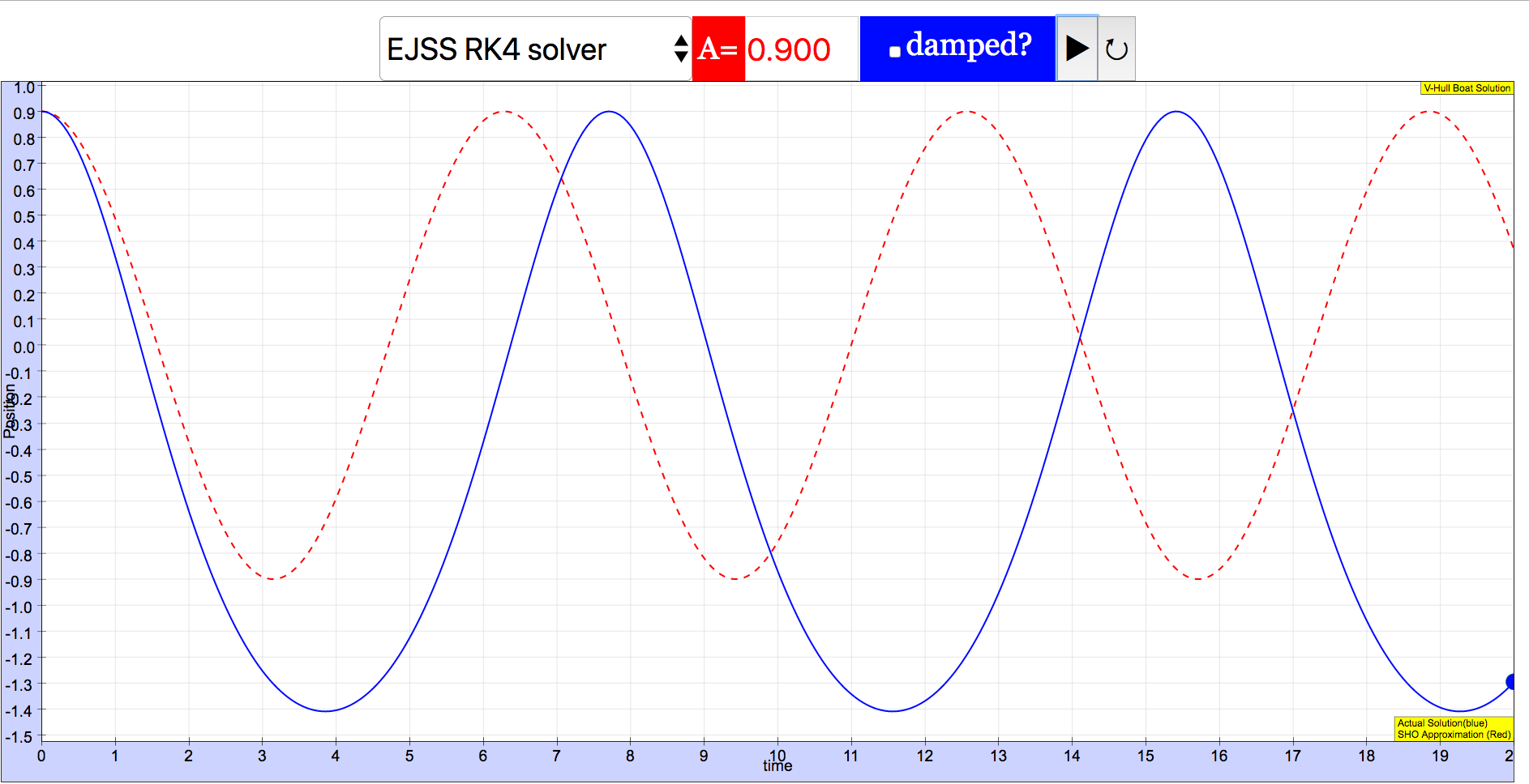
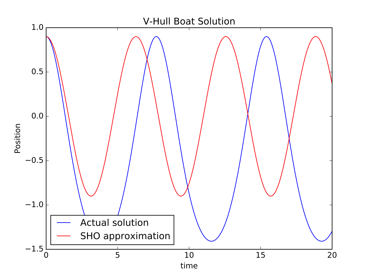
Plot the motion of the boat for various amplitudes. In addition to effects on $T$ , how else does the motion differ from SHO? It will be helpful to plot both the solution to the differential equation and the SHO approximation,

$y (t) = y m a x cos (ω o t) (10)$
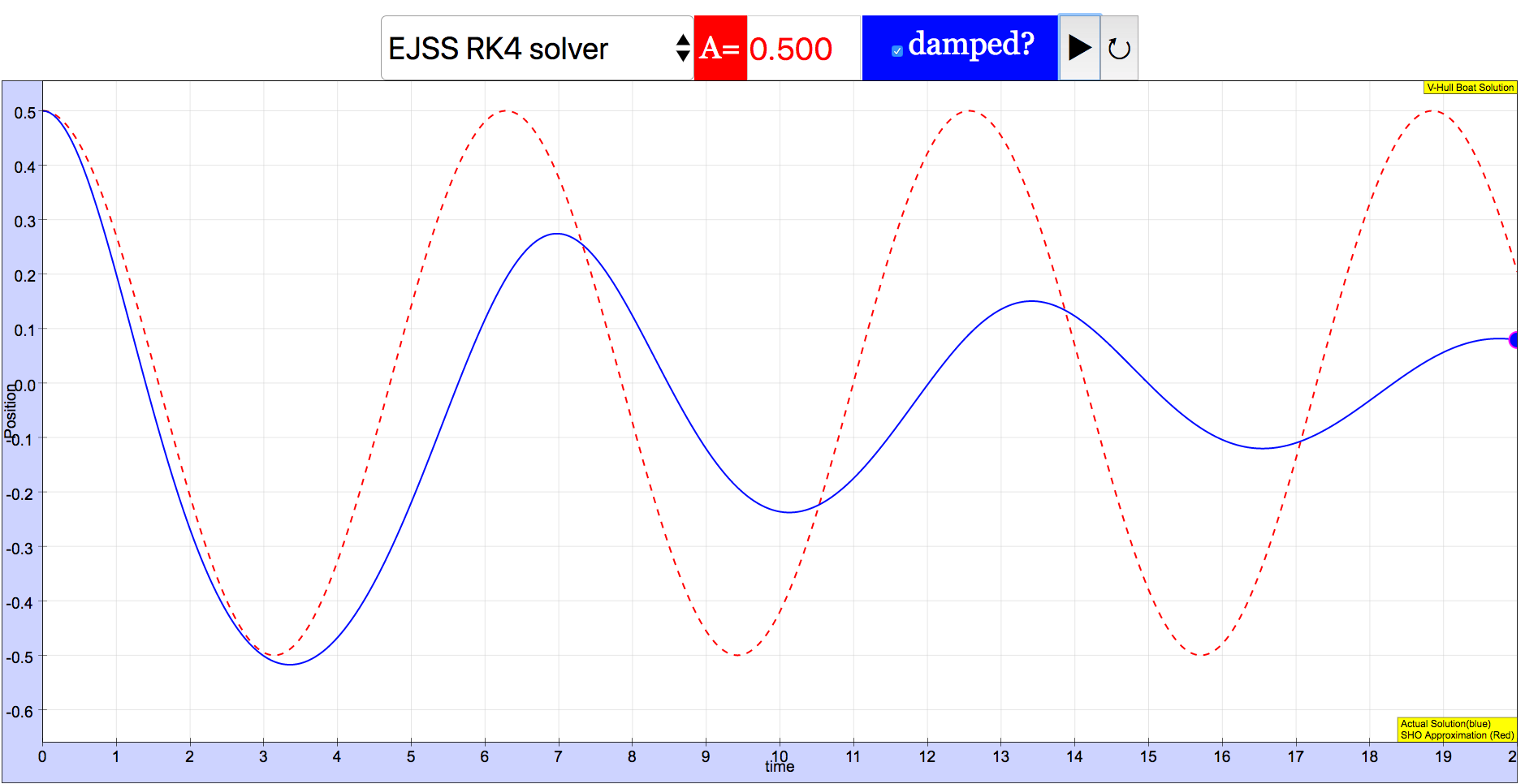
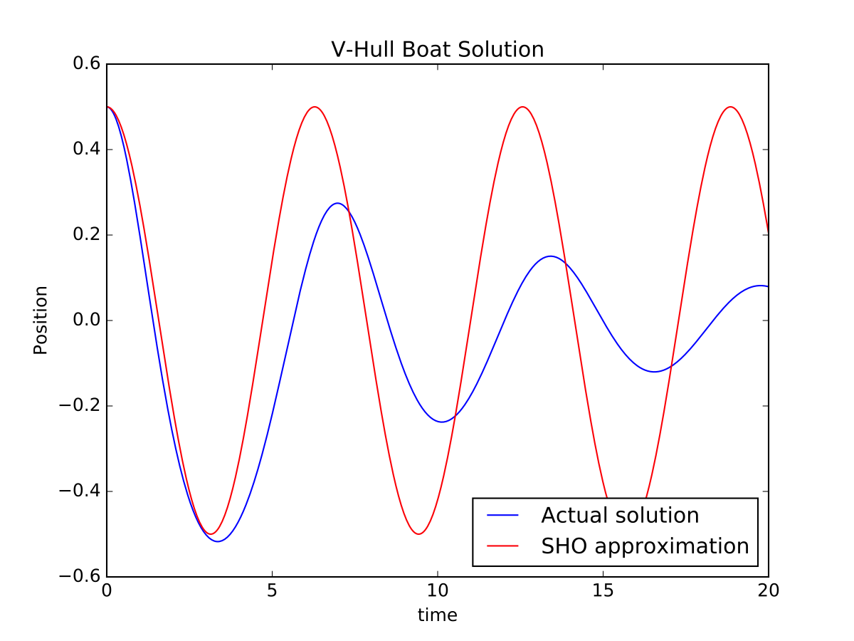
We’ve neglected viscous damping, which is a bad idea in liquids! Redo your calculations, and plots, adding a viscous damping force

$Fv=−δdydt(11)Fv=−δdydt<math xmlns="http://www.w3.org/1998/Math/MathML" display="block"><mtable displaystyle="true"><mlabeledtr><mtd id="mjx-eqn-11"><mtext>(11)</mtext></mtd><mtd><msub><mi>F</mi><mi>v</mi></msub><mo>=</mo><mo>−</mo><mi>δ</mi><mfrac><mrow><mi>d</mi><mi>y</mi></mrow><mrow><mi>d</mi><mi>t</mi></mrow></mfrac></mtd></mlabeledtr></mtable></math>$

to your equations.

vhull.py

#!/usr/bin/env python

'''

vhull.py

Eric Ayars

June 2016

A solution to the vertical motion of a V-hulled boat.

'''

from pylab import *

from scipy.integrate import odeint

# definitions

w = 1.0 # Well, we need to pick something. Might as well

# normalize the frequency. :-)

delta = 0.2 # not sure what this should be, play with it!

def vhull_ODE(s,t):

# derivs function for v-hull ODE, without viscous damping

g0 = s[1]

g1 = -w*(1+s[0]/2)*s[0]

return array([g0,g1])

def vhull_ODE2(s,t):

# derivs function for v-hull ODE, with viscous damping added

g0 = s[1]

g1 = -w*(1+s[0])*s[0] - delta*s[1]

return array([g0,g1])

# Now set up the solutions.

time = linspace(0,20,500) # 500 points on interval [0,20]

# And now plot some things!

# Here's a low-amplitude one, should be approximately SHO.

A = 0.1 # Fairly small amplitude

yi = array([A,0.0])

answer = odeint(vhull_ODE, yi, time)

y = answer[:,0] # position is just the first row

plot(time,y, 'b-', label="Actual solution")

plot(time,A*cos(w*time), 'r-', label="SHO approximation")

A = 0.5 # Not small amplitude

yi = array([A,0.0])

answer = odeint(vhull_ODE, yi, time)

y = answer[:,0] # position is just the first row

plot(time,y, 'b-')

plot(time,A*cos(w*time), 'r-')

'''

# For damped motion, just use vhull_ODE2() instead of vhull_ODE.

A = 0.5

yi = array([A,0.0])

answer = odeint(vhull_ODE2, yi, time)

y = answer[:,0] # position is just the first row

plot(time,y, 'b-', label="Actual solution")

plot(time,A*cos(w*time), 'r-', label="SHO approximation")

'''

title("V-Hull Boat Solution")

xlabel("time")

ylabel("Position")

legend(loc="lower right")

show()

solutions

Exercise 1: A straight-sided boat

For a boat with vertical sides, the equation of motion can be derived by starting with Newton’s second law:

Σ F = m g - ρ g A (y o + y) = m a y (12)

where $A$ is the area of the boat’s cross-section at the waterline. $y_{o}$ is the equilibrium depth, so $m g = ρ g A y_{o}$ and

ay=d2ydt2=−ρgAmy(13)ay=d2ydt2=−ρgAmy<math xmlns="http://www.w3.org/1998/Math/MathML" display="block"><mtable displaystyle="true"><mlabeledtr><mtd id="mjx-eqn-13"><mtext>(13)</mtext></mtd><mtd><msub><mi>a</mi><mi>y</mi></msub><mo>=</mo><mfrac><mrow><msup><mi>d</mi><mn>2</mn></msup><mi>y</mi></mrow><mrow><mi>d</mi><msup><mi>t</mi><mn>2</mn></msup></mrow></mfrac><mo>=</mo><mo>−</mo><mfrac><mrow><mi>ρ</mi><mi>g</mi><mi>A</mi></mrow><mi>m</mi></mfrac><mi>y</mi></mtd></mlabeledtr></mtable></math>

This is in the form of the equation for SHO, with

ω=ρgAm−−−−√(14)ω=√ρgAm<math xmlns="http://www.w3.org/1998/Math/MathML" display="block"><mtable displaystyle="true"><mlabeledtr><mtd id="mjx-eqn-14"><mtext>(14)</mtext></mtd><mtd><mi>ω</mi><mo>=</mo><msqrt><mfrac><mrow><mi>ρ</mi><mi>g</mi><mi>A</mi></mrow><mi>m</mi></mfrac></msqrt></mtd></mlabeledtr></mtable></math>

The period of the boat’s oscillation will be

T=2πmρgA−−−−√(15)T=2π√mρgA<math xmlns="http://www.w3.org/1998/Math/MathML" display="block"><mtable displaystyle="true"><mlabeledtr><mtd id="mjx-eqn-15"><mtext>(15)</mtext></mtd><mtd><mi>T</mi><mo>=</mo><mn>2</mn><mi>π</mi><msqrt><mfrac><mi>m</mi><mrow><mi>ρ</mi><mi>g</mi><mi>A</mi></mrow></mfrac></msqrt></mtd></mlabeledtr></mtable></math>

Exercise 2: A V-hulled boat

The derivation for the V-hulled boat follows the same general procedure.

V=12βh2L=12βL(yo+y)2(16)V=12βh2L=12βL(yo+y)2<math xmlns="http://www.w3.org/1998/Math/MathML" display="block"><mtable displaystyle="true"><mlabeledtr><mtd id="mjx-eqn-16"><mtext>(16)</mtext></mtd><mtd><mi>V</mi><mo>=</mo><mfrac><mn>1</mn><mn>2</mn></mfrac><mi>β</mi><msup><mi>h</mi><mn>2</mn></msup><mi>L</mi><mo>=</mo><mfrac><mn>1</mn><mn>2</mn></mfrac><mi>β</mi><mi>L</mi><mo stretchy="false">(</mo><msub><mi>y</mi><mi>o</mi></msub><mo>+</mo><mi>y</mi><msup><mo stretchy="false">)</mo><mn>2</mn></msup></mtd></mlabeledtr></mtable></math>

ΣF=md2ydt2=mg−12ρgβL(y2o+2yoy+y2)(17)ΣF=md2ydt2=mg−12ρgβL(y2o+2yoy+y2)<math xmlns="http://www.w3.org/1998/Math/MathML" display="block"><mtable displaystyle="true"><mlabeledtr><mtd id="mjx-eqn-17"><mtext>(17)</mtext></mtd><mtd><mi mathvariant="normal">Σ</mi><mi>F</mi><mo>=</mo><mi>m</mi><mfrac><mrow><msup><mi>d</mi><mn>2</mn></msup><mi>y</mi></mrow><mrow><mi>d</mi><msup><mi>t</mi><mn>2</mn></msup></mrow></mfrac><mo>=</mo><mi>m</mi><mi>g</mi><mo>−</mo><mfrac><mn>1</mn><mn>2</mn></mfrac><mi>ρ</mi><mi>g</mi><mi>β</mi><mi>L</mi><mrow><mo>(</mo><mrow><msubsup><mi>y</mi><mi>o</mi><mn>2</mn></msubsup><mo>+</mo><mn>2</mn><msub><mi>y</mi><mi>o</mi></msub><mi>y</mi><mo>+</mo><msup><mi>y</mi><mn>2</mn></msup></mrow><mo>)</mo></mrow></mtd></mlabeledtr></mtable></math>

The equilibrium position is given by $y_{o}$ , so $m g - \frac{1}{2} ρ g β L y_{o}^{2} = 0$ and

d2ydt2=−ρgβL2m(2yoy+y2)(18)d2ydt2=−ρgβL2m(2yoy+y2)<math xmlns="http://www.w3.org/1998/Math/MathML" display="block"><mtable displaystyle="true"><mlabeledtr><mtd id="mjx-eqn-18"><mtext>(18)</mtext></mtd><mtd><mfrac><mrow><msup><mi>d</mi><mn>2</mn></msup><mi>y</mi></mrow><mrow><mi>d</mi><msup><mi>t</mi><mn>2</mn></msup></mrow></mfrac><mo>=</mo><mo>−</mo><mfrac><mrow><mi>ρ</mi><mi>g</mi><mi>β</mi><mi>L</mi></mrow><mrow><mn>2</mn><mi>m</mi></mrow></mfrac><mrow><mo>(</mo><mrow><mn>2</mn><msub><mi>y</mi><mi>o</mi></msub><mi>y</mi><mo>+</mo><msup><mi>y</mi><mn>2</mn></msup></mrow><mo>)</mo></mrow></mtd></mlabeledtr></mtable></math>

This can be further simplified as

d2ydt2=−ρgβLyom(1+y2yo)y(19)d2ydt2=−ρgβLyom(1+y2yo)y<math xmlns="http://www.w3.org/1998/Math/MathML" display="block"><mtable displaystyle="true"><mlabeledtr><mtd id="mjx-eqn-19"><mtext>(19)</mtext></mtd><mtd><mfrac><mrow><msup><mi>d</mi><mn>2</mn></msup><mi>y</mi></mrow><mrow><mi>d</mi><msup><mi>t</mi><mn>2</mn></msup></mrow></mfrac><mo>=</mo><mo>−</mo><mfrac><mrow><mi>ρ</mi><mi>g</mi><mi>β</mi><mi>L</mi><msub><mi>y</mi><mi>o</mi></msub></mrow><mi>m</mi></mfrac><mrow><mo>(</mo><mrow><mn>1</mn><mo>+</mo><mfrac><mi>y</mi><mrow><mn>2</mn><msub><mi>y</mi><mi>o</mi></msub></mrow></mfrac></mrow><mo>)</mo></mrow><mi>y</mi></mtd></mlabeledtr></mtable></math>

From that equation we can see that if $\frac{y}{2 y_{o}}$ is small, then the motion is approximately SHO with

ωo=ρgβLyom−−−−−−−√(20)ωo=√ρgβLyom<math xmlns="http://www.w3.org/1998/Math/MathML" display="block"><mtable displaystyle="true"><mlabeledtr><mtd id="mjx-eqn-20"><mtext>(20)</mtext></mtd><mtd><msub><mi>ω</mi><mi>o</mi></msub><mo>=</mo><msqrt><mfrac><mrow><mi>ρ</mi><mi>g</mi><mi>β</mi><mi>L</mi><msub><mi>y</mi><mi>o</mi></msub></mrow><mi>m</mi></mfrac></msqrt></mtd></mlabeledtr></mtable></math>

There are an awful lot of constants in that equation, so to simplify our numeric calculations let’s just redefine things.

d2ydt2=−ω2o(1+y2yo)y(21)d2ydt2=−ω2o(1+y2yo)y<math xmlns="http://www.w3.org/1998/Math/MathML" display="block"><mtable displaystyle="true"><mlabeledtr><mtd id="mjx-eqn-21"><mtext>(21)</mtext></mtd><mtd><mfrac><mrow><msup><mi>d</mi><mn>2</mn></msup><mi>y</mi></mrow><mrow><mi>d</mi><msup><mi>t</mi><mn>2</mn></msup></mrow></mfrac><mo>=</mo><mo>−</mo><msubsup><mi>ω</mi><mi>o</mi><mn>2</mn></msubsup><mrow><mo>(</mo><mrow><mn>1</mn><mo>+</mo><mfrac><mi>y</mi><mrow><mn>2</mn><msub><mi>y</mi><mi>o</mi></msub></mrow></mfrac></mrow><mo>)</mo></mrow><mi>y</mi></mtd></mlabeledtr></mtable></math>

We can also define the unitless variable $γ \equiv \frac{y}{y_{o}}$ , which allows us to rewrite the equation in (almost) unit-independent form:

d2γdt2=−ω2o(1+γ2)γ(22)d2γdt2=−ω2o(1+γ2)γ<math xmlns="http://www.w3.org/1998/Math/MathML" display="block"><mtable displaystyle="true"><mlabeledtr><mtd id="mjx-eqn-22"><mtext>(22)</mtext></mtd><mtd><mfrac><mrow><msup><mi>d</mi><mn>2</mn></msup><mi>γ</mi></mrow><mrow><mi>d</mi><msup><mi>t</mi><mn>2</mn></msup></mrow></mfrac><mo>=</mo><mo>−</mo><msubsup><mi>ω</mi><mi>o</mi><mn>2</mn></msubsup><mrow><mo>(</mo><mrow><mn>1</mn><mo>+</mo><mfrac><mi>γ</mi><mn>2</mn></mfrac></mrow><mo>)</mo></mrow><mi>γ</mi></mtd></mlabeledtr></mtable></math>

That’s the equation we need to send through the ODE solver.

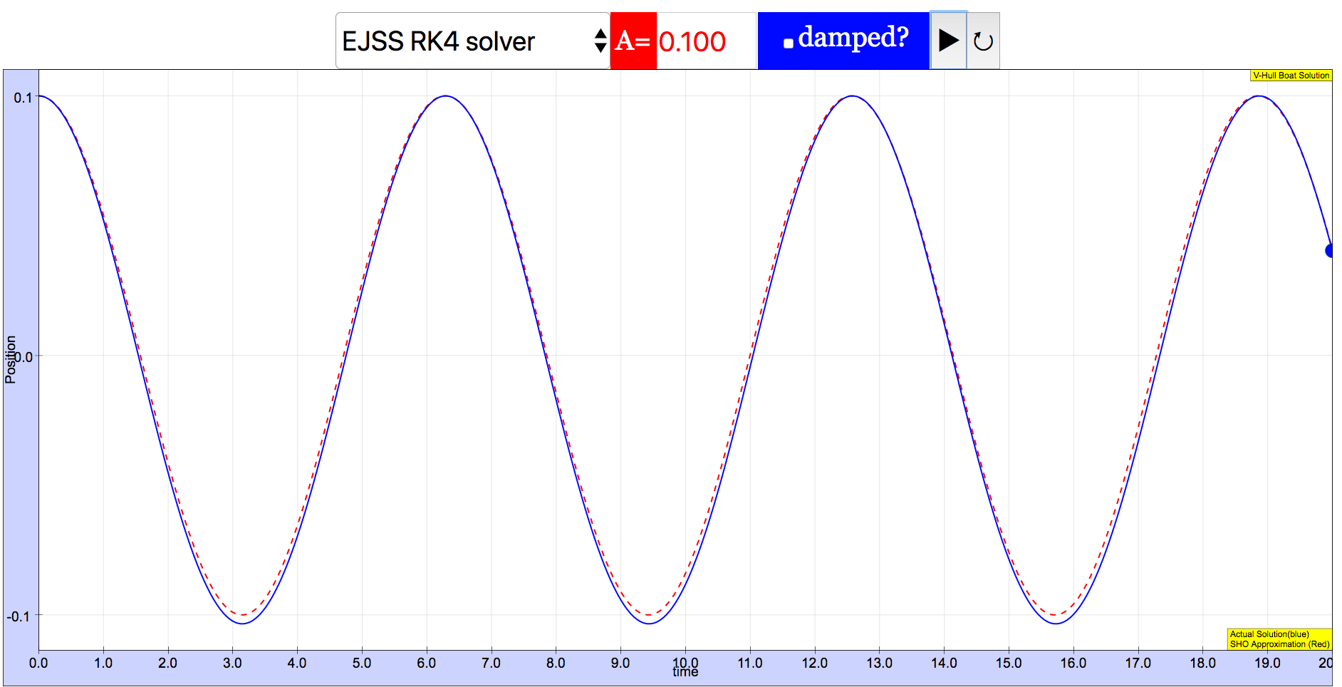
The equation is approximately SHO if the amplitude is small. The easist way to control the amplitude is to set initial position to $y_{i}$ , with $v_{i} = 0$ , so that the amplitude is $y_{i}$ .

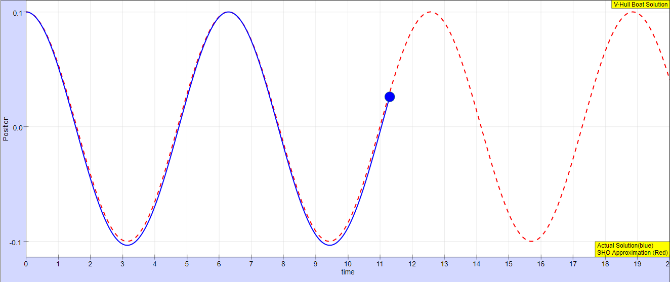
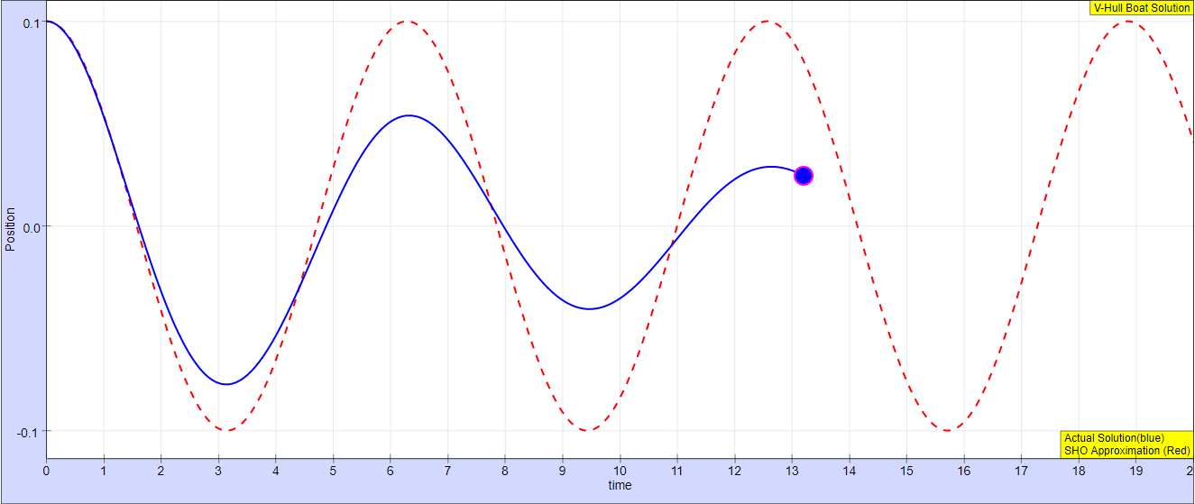
Setting different values of amplitude gives different behavior: for small amplitude ( $γ_{o} = 0.1$ ) the result is nearly indistinguishable from SHO, but for larger values both the period and symmetry change. The figure below shows that at $γ_{o} = 0.5$ , the boat spends more time higher (the graph is inverted, since down is positive in our initial setup) and the period lengthens relative to the SHO approximation.

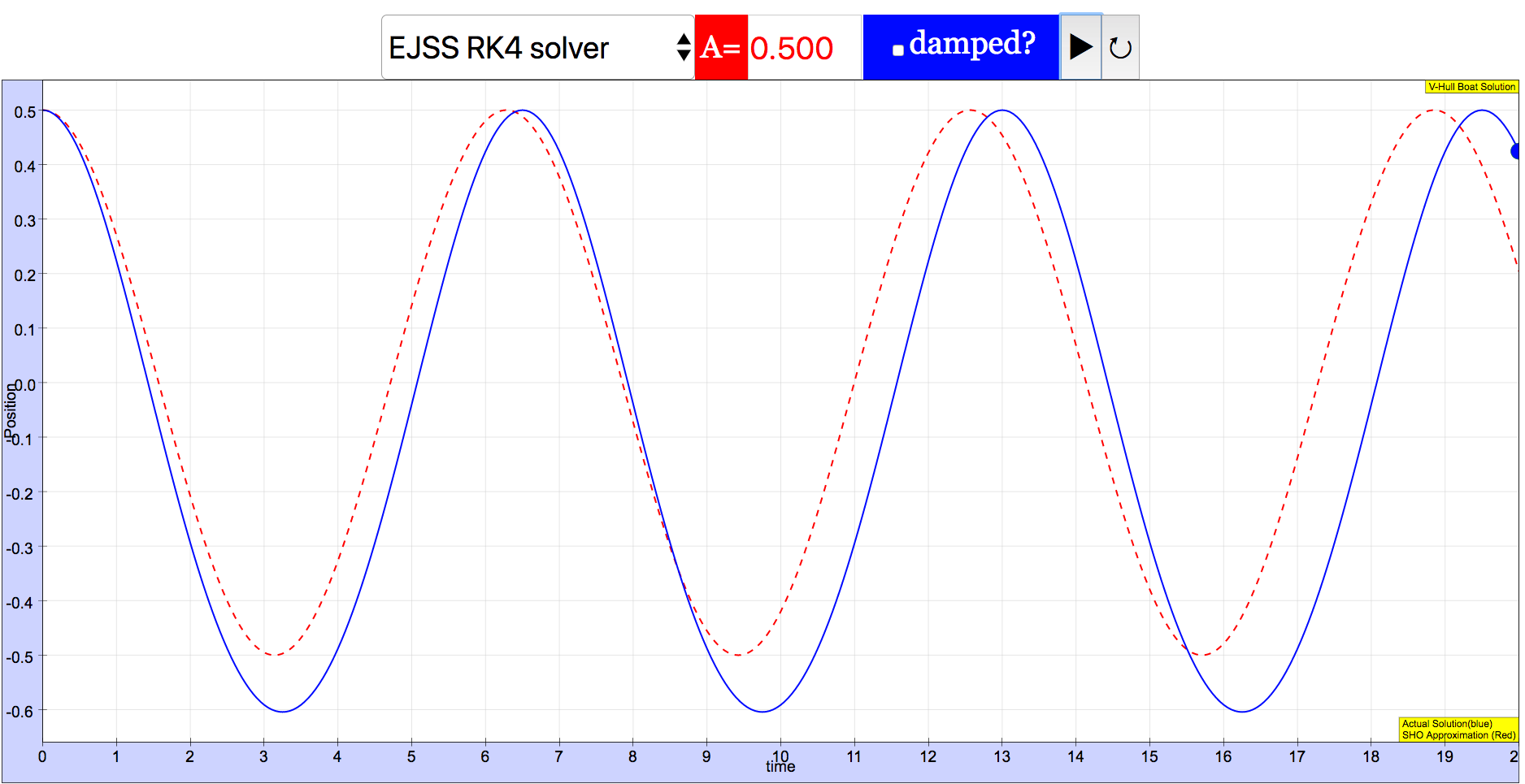
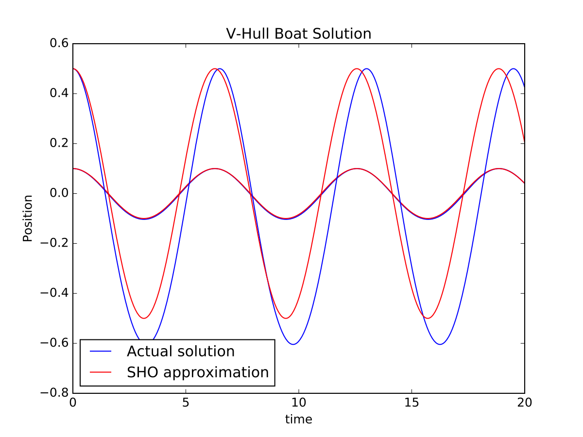
Solution to the V-hull boat oscillation

These effects are even more prominent at larger values of $γ_{o}$ , as shown in the next figure.

Solution to the V-hull boat oscillation at large amplitude

There’s an opportunity here for the model to break down. If the boat gets completely out of the water, then the width of the boat becomes negative (ok, it doesn’t really but it does in the model) so then the volume becomes negative and the buoyant force becomes negative and the boat leaps away from the water exactly the way that real boats don’t. Be prepared to discuss this interesting result should the students get the amplitude too high.

Adding damping is relatively easy: just add another force term in the definition of the ODE. Results are shown below.

Solution to the V-hull boat oscillation with damping

Translations

Code	Language		Translator	Run

Credits

Fremont Teng; Loo Kang Wee

http://iwant2study.org/lookangejss/02_newtonianmechanics_8oscillations/ejss_model_PICUP_vhull_frem_v2/)

Executive Summary:

This document reviews an open educational resource focused on exploring harmonic and anharmonic oscillations using a boat as a model. The resource, developed by E. Ayars with Easy JavaScript Simulation by Fremont Teng and Loo Kang Wee, provides exercises that guide students to understand the behavior of an anharmonic oscillator, particularly the asymmetric oscillation of a V-hulled boat. The core idea is to contrast this with the well-understood Simple Harmonic Oscillation (SHO) and to identify conditions under which anharmonic motion can be approximated as SHO. The resource utilizes computational tools like ODE solvers (with suggested implementations in Python and Mathematica) and includes a JavaScript simulation applet for interactive exploration.

Main Themes and Important Ideas/Facts:

Introduction to Anharmonic Oscillations: The resource introduces the concept of anharmonic oscillation as a more general form of periodic motion beyond the familiar Simple Harmonic Oscillation (SHO). It highlights that while SHO is simple and has known solutions, many real-world systems exhibit anharmonic behavior.
"Simple Harmonic Oscillation (SHO) is everyone’s favorite type of periodic motion. It’s simple, easy to understand, and has a known solution. But SHO is not the only kind of periodic motion. In this set of exercises we’ll investigate an anharmonic oscillator."
Idealized Boat Hull as an Anharmonic Oscillator: The exercises focus on an idealized boat hull, specifically a V-hulled boat, as a system that demonstrates asymmetric oscillation. The restoring force in such a system is stronger for displacements in one direction compared to the other, leading to non-sinusoidal oscillations for large amplitudes.
"Here we investigate an idealized boat hull which exhibits asymmetric oscillation: the restoring force is stronger for displacements in one direction than in the other. This results, for large oscillations, in a visibly non-sinusoidal oscillation."
Approximation of Anharmonic Motion as SHO for Small Oscillations: A key concept explored is that even anharmonic oscillators can often be approximated as SHO when the oscillations are small. This is demonstrated in the case of the V-hulled boat.
"For small oscillations, the motion is approximately simple harmonic again." "This is not SHO! If γ is small, it is approximately SHO, but only approximately."
Mathematical Modeling using Differential Equations: The resource emphasizes using differential equations to model the motion of the boat. It presents the equation of motion for both a straight-sided boat (resulting in SHO) and a V-hulled boat (resulting in anharmonic oscillation).
For the straight-sided boat: "d²y/dt² = − (ρgA/m) y" which is in the form of SHO. For the V-hulled boat (in a simplified form): "d²γ/dt² = − ω²₀ (1 + γ²) γ" which is identified as not SHO.
The Role of ODE Solvers: The exercises guide students to use Ordinary Differential Equation (ODE) solvers to analyze the behavior of the anharmonic oscillator. This allows for a qualitative understanding of the motion, especially for cases where analytical solutions are not straightforward. The resource mentions Python and Mathematica as available implementations and suggests that instructors could incorporate real physical parameters.
"Students who complete these exercises will be able to use an ODE solver to develop a qualitative understanding of the behavior of an anharmonic oscillator." "This set of exercises guides students through the development of an anharmonic oscillator, then lets them use an ODE solver to plot the motion. It does not describe how to use an ODE solver. Emphasis is on qualitative understanding of the system..."
Qualitative Understanding of Anharmonic Motion: The focus is on gaining a qualitative understanding of how anharmonic oscillation differs from SHO. This includes observing changes in the period and the sinusoidal nature of the motion, particularly at larger amplitudes. The resource notes that for a V-hulled boat with larger oscillations, the period lengthens, and the motion becomes asymmetric.
"Setting different values of amplitude gives different behavior: for small amplitude (γ₀ = 0.1) the result is nearly indistinguishable from SHO, but for larger values both the period and symmetry change. The figure below shows that at γ₀ = 0.5, the boat spends more time higher (the graph is inverted, since down is positive in our initial setup) and the period lengthens relative to the SHO approximation."
Limitations of the Model: The resource explicitly points out the limitations of the idealized model, especially when the amplitude of oscillation becomes too large, causing the boat to theoretically leave the water in a non-physical way within the model. This provides an opportunity for discussing the scope and validity of physical models.
"In this problem, if the amplitude is high enough that the boat gets out of the water, the model in the ODE breaks down in interesting and spectacular ways."
Effect of Damping: The exercises also encourage the inclusion of viscous damping forces in the model to make it more realistic, acknowledging that damping is significant in liquids. This allows students to observe how damping affects both SHO and anharmonic oscillations.
"We’ve neglected viscous damping, which is a bad idea in liquids! Redo your calculations, and plots, adding a viscous damping force Fv = − δ dy/dt to your equations."
Interactive JavaScript Simulation: The resource includes an embedded Easy JavaScript Simulation applet, providing an interactive way for students to explore harmonic and anharmonic oscillations of a boat. The simulation allows users to adjust parameters like amplitude and toggle damping, and it includes a playable animation using the EJSS RK4 Solver.

Exercises:

The resource includes two main exercises:

Exercise 1: A straight-sided boat: This exercise guides students to show that the vertical motion of a straight-sided boat is SHO and to determine its period.
Exercise 2: A V-hulled boat: This exercise requires students to demonstrate that the vertical motion of a V-hulled boat is not SHO, to find the approximate SHO frequency for small oscillations, and to investigate the behavior for larger oscillations using numerical solutions and plots. It also asks students to consider the effect of viscous damping.

Target Audience and Learning Objectives:

The resource is designed for first-year university students and beyond, in subject areas related to mechanics and oscillations. The learning objectives include enabling students to:

Develop a qualitative understanding of the behavior of an anharmonic oscillator.
Use an ODE solver to model and analyze physical systems.
Understand the conditions under which anharmonic motion can be approximated as simple harmonic.
Explore the differences between harmonic and anharmonic oscillations.

Computational Tools:

The resource suggests the use of built-in differential equation solving capabilities in Python (using scipy.integrate.odeint as shown in the provided vhull.py code) and Mathematica. It also mentions that for other implementations, resources like "Numerical Recipes in C" can provide guidance on finite-difference methods.

Overall Assessment:

This resource provides a valuable and engaging way for students to learn about harmonic and, more importantly, anharmonic oscillations. By using the relatable example of a boat and incorporating computational tools and a simulation, it moves beyond the purely theoretical treatment often found in introductory physics. The exercises are structured to guide students through the process of modeling, analyzing, and understanding the nuances of non-simple periodic motion. The explicit discussion of the model's limitations is a strength, encouraging critical thinking about the applicability of theoretical models. The inclusion of a JavaScript simulation enhances the learning experience by providing an interactive and visual tool for exploration.

Study Guide: Harmonic and Anharmonic Oscillations of a Boat

Key Concepts

Simple Harmonic Oscillation (SHO): A type of periodic motion where the restoring force is directly proportional to the displacement and acts in the opposite direction. Its equation of motion is of the form $d^2x/dt^2 = -\omega^2 x$ , resulting in sinusoidal oscillations.
Anharmonic Oscillation: Periodic motion where the restoring force is not directly proportional to the displacement. The equation of motion cannot be simplified to the standard SHO form, leading to non-sinusoidal oscillations.
Restoring Force: A force that acts to bring a system back to its equilibrium position after it has been displaced.
Equation of Motion: A mathematical equation that describes the motion of a physical system in terms of its position, velocity, acceleration, and the forces acting upon it. For oscillatory systems, it relates the acceleration to the displacement.
Equilibrium Position: The position where the net force on an object is zero, and the object remains at rest if undisturbed.
Buoyant Force: The upward force exerted by a fluid that opposes the weight of an immersed object. Its magnitude is equal to the weight of the fluid displaced by the object (Archimedes' principle).
ODE Solver: A numerical method or software used to find approximate solutions to ordinary differential equations, particularly when analytical solutions are difficult or impossible to obtain.
Angular Frequency (ω): A measure of the rate of oscillation, related to the frequency (f) and period (T) by $\omega = 2\pi f = 2\pi/T$ .
Period (T): The time taken for one complete cycle of an oscillation.
Amplitude: The maximum displacement from the equilibrium position during an oscillation.
Viscous Damping: A force that opposes the motion of an object moving through a fluid, proportional to the velocity of the object. It causes the amplitude of oscillations to decrease over time.
Approximation: A simplified model or solution that is valid under certain conditions, such as small displacements.

Quiz

What is the defining characteristic of Simple Harmonic Oscillation (SHO), and what mathematical form does its equation of motion take?
Explain the difference between a harmonic oscillator and an anharmonic oscillator based on their restoring forces and resulting motion.
In the context of the straight-sided boat example, what are the two main forces acting on the boat, and under what condition is the boat in equilibrium?
How is the buoyant force on the straight-sided boat related to the volume of water displaced, and how does this volume change when the boat is displaced vertically?
Describe why the vertical motion of a straight-sided boat is considered Simple Harmonic Oscillation. What form does its angular frequency take?
For the V-hulled boat, how does the width of the hull at the waterline depend on the depth below the waterline, and how does this affect the volume of water displaced?
Explain why the vertical motion of the V-hulled boat is not Simple Harmonic Oscillation, as shown by its equation of motion.
Under what condition can the motion of the V-hulled boat be approximated as Simple Harmonic Oscillation, and what is the approximate angular frequency in this case?
According to the text, how does increasing the amplitude of oscillation affect the period and symmetry of the V-hulled boat's motion compared to the SHO approximation?
What effect does adding viscous damping have on the oscillations of the V-hulled boat, and how is this force typically modeled mathematically?

Quiz Answer Key

Simple Harmonic Oscillation is characterized by a restoring force that is directly proportional to the displacement and acts in the opposite direction. Its equation of motion has the form $d^2x/dt^2 = -\omega^2 x$ , where $\omega^2$ is a positive constant.
In a harmonic oscillator, the restoring force is linearly proportional to the displacement, resulting in sinusoidal motion. In an anharmonic oscillator, this proportionality does not hold, leading to non-sinusoidal oscillations where the period and shape can depend on the amplitude.
The two main forces acting on the straight-sided boat are its weight ( $mg$ ) acting downwards and the buoyant force ( $-\rho g V$ ) acting upwards. The boat is in equilibrium when these two forces are balanced, meaning the weight equals the buoyant force.
The buoyant force is equal to the negative weight of the water displaced, $-\rho g V$ . For a straight-sided boat with cross-sectional area $A$ , if the equilibrium depth is $x_o$ , then $V = A(x_o + x)$ when displaced by $x$ .
The equation of motion for the straight-sided boat derived in the text is $d^2y/dt^2 = -(\rho g A / m) y$ , which matches the form of the SHO equation. Therefore, the motion is SHO with an angular frequency $\omega = \sqrt{\rho g A / m}$ .
For the V-hulled boat, the width of the hull at the waterline ( $w$ ) is proportional to the depth below the waterline ( $h$ ), given by $w = \beta h$ . This V-shape causes the volume of displaced water to be proportional to the square of the depth ( $V = \frac{1}{2} \beta h^2 L$ ).
The equation of motion for the V-hulled boat is $d^2 y / dt^2 = - \omega_o^2 (1 + y / (2 y_o)) y$ or $d^2 \gamma / dt^2 = - \omega_o^2 (1 + \gamma / 2) \gamma$ (using one form from the python code), which includes a term proportional to $y^2$ , thus not fitting the linear form of SHO. This non-linearity makes the oscillation anharmonic. (Note: The provided text has slightly different forms of this equation in the theory and solutions sections, but the key is the presence of non-linear terms in $y$ ).
The motion of the V-hulled boat can be approximated as SHO when the term $y / (2 y_o)$ (or $\gamma / 2$ ) is small, meaning the amplitude of oscillation $y$ is much smaller than the equilibrium depth $y_o$ . In this case, the approximate angular frequency is $\omega_o = \sqrt{\rho g \beta L y_o / m}$ .
For larger amplitudes, the period of the V-hulled boat's oscillation lengthens relative to the SHO approximation. Additionally, the motion becomes asymmetric, with the boat spending more time at higher positions (less submerged in the original setup where down is positive).
Adding viscous damping introduces a force that opposes the velocity of the boat, typically modeled as $F_v = -\delta dy/dt$ . This force causes the amplitude of the oscillations to decay exponentially over time.

Essay Format Questions

Compare and contrast the derivation of the equation of motion for the straight-sided boat and the V-hulled boat. What are the key differences in the assumptions and the resulting mathematical forms, and how do these differences explain the nature of their oscillations?
Discuss the concept of approximating anharmonic motion as Simple Harmonic Oscillation. Under what conditions is this approximation valid for the V-hulled boat, and what are the limitations and consequences of using this approximation for larger oscillations?
Explain how the V-shaped hull of the boat leads to anharmonic oscillations. How does the restoring force in this system differ from the linear restoring force in Simple Harmonic Motion, and how does this affect the period and shape of the oscillations?
The text mentions the potential breakdown of the V-hulled boat model at very high amplitudes. Describe this breakdown and explain why it occurs within the context of the model's assumptions about the buoyant force. How does this highlight the limitations of idealized physical models?
Analyze the effect of viscous damping on the oscillations of the V-hulled boat. How does damping alter the equation of motion, and what are the observable differences in the boat's motion over time with and without damping? Discuss the realism of including a damping term in this physical model.

Glossary of Key Terms

Anharmonic Oscillator: A system that oscillates periodically but whose restoring force is not directly proportional to its displacement from equilibrium, leading to non-sinusoidal motion.
Buoyant Force: The upward force exerted by a fluid that opposes the weight of an immersed object; equal to the weight of the fluid displaced by the object (Archimedes' Principle).
Damping: A process that dissipates energy from an oscillating system, usually through friction or resistance, causing the amplitude of oscillations to decrease over time.
Equation of Motion: A mathematical expression that describes the behavior of a physical system as a function of time, usually relating forces, masses, and accelerations (Newton's laws) or energy.
Equilibrium: A state in which the net force acting on an object or system is zero, resulting in no acceleration. For oscillations, it is the position about which the motion occurs.
Harmonic Oscillator: A system that, when displaced from its equilibrium position, experiences a restoring force directly proportional to the displacement; it undergoes Simple Harmonic Motion.
ODE Solver: A numerical algorithm used to find approximate solutions to ordinary differential equations, often employed when analytical solutions are not feasible.
Oscillation: A repetitive variation, typically in time, of some measure about a central value or between two or more different states.
Period (T): The duration of one complete cycle in a repetitive event, such as an oscillation or a wave.
Restoring Force: A force that acts to bring a displaced object or system back towards its equilibrium position.
Simple Harmonic Motion (SHO): A type of periodic motion where the restoring force is directly proportional to the displacement and acts in the direction opposite to that of displacement, resulting in sinusoidal oscillations.
Viscous Damping: A type of damping force that is proportional to the velocity of the moving object and opposes its motion, often occurring when an object moves through a fluid.

Sample Learning Goals

[text]

For Teachers

Instructions

Solver Combo Box

Toggle this combo box to select their respective solver.

Selecting the EJSS RK4 Solver includes a playable animation.

Amplitude Field Box

Adjust this to change the amplitude of the wave.

Damped Check Box

Toggling this will determine if the oscillation is damped or not.

(Not Damped)

(Damped)

Play/Pause and Reset Buttons

Plays/Pauses and resets the simulation respectively.

That is all, do enjoy the simulation in the link below:

http://iwant2study.org/lookangejss/02_newtonianmechanics_8oscillations/ejss_model_PICUP_vhull_frem_v2/

Research

[text]

Video

[text]

Version:

Other Resources

[text]

Frequently Asked Questions: Harmonic and Anharmonic Oscillations of a Boat

1. What is the difference between harmonic and anharmonic oscillation?

Simple Harmonic Oscillation (SHO) is a periodic motion where the restoring force is directly proportional to the displacement from the equilibrium position, resulting in a sinusoidal motion over time. Anharmonic oscillation, on the other hand, occurs when the restoring force is not directly proportional to the displacement, leading to non-sinusoidal and often asymmetric oscillations.

2. How does a straight-sided boat exhibit Simple Harmonic Oscillation (SHO)?

When a straight-sided boat is displaced vertically from its equilibrium, the buoyant force changes linearly with the additional submerged volume (which is directly proportional to the displacement). This linear restoring force leads to an equation of motion that is mathematically identical to that of a mass on a spring, thus resulting in SHO with a specific angular frequency and period determined by the boat's mass and the water's density and the boat's cross-sectional area at the waterline.

3. Why does a V-hulled boat exhibit anharmonic oscillation for larger amplitudes?

For a V-hulled boat, the width at the waterline, and consequently the volume of displaced water and the buoyant force, changes non-linearly with the depth of submersion. This non-linear relationship between the restoring force and the displacement, especially for larger vertical displacements, results in an equation of motion that deviates from the form of SHO, making the oscillations anharmonic. The restoring force becomes stronger in one direction of displacement compared to the other.

4. Under what conditions can the motion of a V-hulled boat be approximated as Simple Harmonic Oscillation (SHO)?

The motion of a V-hulled boat can be approximated as SHO when the oscillations are small. In this case, the non-linear terms in the equation of motion become negligible compared to the linear term, making the restoring force approximately proportional to the displacement. This approximation is valid when the square of the displacement is much smaller than twice the equilibrium depth ( $y^2 << 2y_o$ ).

5. How does the period of oscillation of a V-hulled boat change with larger amplitudes compared to the SHO approximation?

For a V-hulled boat, as the amplitude of oscillation increases beyond the small oscillation regime, the period of oscillation typically lengthens compared to the period predicted by the SHO approximation ( $\text{T}_o = 2\pi/\omega_o$ ). This is because the non-linear restoring force alters the time it takes for a complete cycle of motion.

6. Besides the period, how else does the motion of a V-hulled boat with large amplitudes differ from SHO?

In addition to the change in period, the motion of a V-hulled boat with large amplitudes differs from SHO in its shape. The oscillations become visibly non-sinusoidal and asymmetric. The boat may spend more time at higher or lower positions depending on the asymmetry of the restoring force, and the peaks and troughs of the motion are no longer as smooth and predictable as in a perfect sine wave.

7. What are some limitations of the idealized V-hulled boat model presented?

One significant limitation discussed is the breakdown of the model at very large amplitudes where the boat can get completely out of the water. In such a scenario, the model incorrectly predicts a negative buoyant force and a rapid upward acceleration, which does not physically occur. The model also neglects viscous damping from the water, which would, in reality, cause the oscillations to decrease in amplitude over time.

8. How can viscous damping be incorporated into the model of the oscillating boats?

Viscous damping, which represents the resistance to motion caused by the fluid (water), can be incorporated into the equations of motion by adding a force term that is proportional to and in the opposite direction of the velocity of the boat ( $F_v = -\delta \frac{dy}{dt}$ ). This additional term introduces a damping effect, causing the amplitude of oscillations to decay exponentially over time. Including this term provides a more realistic representation of the boat's motion in water.

1 1 1 1 1 1 1 1 1 1 Rating 0.00 (0 Votes)

Details: Written by Loo Kang Wee; Parent Category: 02 Newtonian Mechanics; Category: 09 Oscillations; Published: 18 July 2018; Created: 18 July 2018; Last Updated: 22 March 2025; Hits: 4300

RSS Feed

Breadcrumbs