
.png
)


About
Developed by W. Freeman
The standard description of the behavior of the vibrating string is only valid in the low-amplitude limit. In this exercise, students build a lattice-elasticity model of a vibrating string and then study its properties, first verifying that the standard properties predicted by hold in the low-amplitude limit and then studying the nonlinear properties of the vibrating string as the amplitude increases.
| Subject Areas | Waves & Optics, Mathematical/Numerical Methods, and Other |
|---|---|
| Levels | Beyond the First Year and Advanced |
| Available Implementation | C/C++ |
| Learning Objectives |
|
| Time to Complete | 90-360 min |
#include <stdio.h>
#include <stdlib.h>
#include <math.h>
#include <time.h>
// #define ONE_PERIOD_ONLY // uncomment this to do only one period, then print stats and exit.
void get_forces(double *x, double *y, double *Fx, double *Fy, int N, double k, double r0) // pointers here are array parameters
{
int i;
double r;
Fx[0]=Fy[0]=Fx[N]=Fy[N]=0; // have to set the end forces properly to avoid possible uninitialized memory shenanigans
double U=0,E=0,T=0;
for (i=1;i<N;i++)
{
// left force
r = hypot(x[i]-x[i-1],y[i]-y[i-1]);
Fx[i] = -(x[i]-x[i-1]) * k * (r-r0)/r;
Fy[i] = -(y[i]-y[i-1]) * k * (r-r0)/r;
// right force
r = hypot(x[i]-x[i+1],y[i]-y[i+1]);
Fx[i] += -(x[i]-x[i+1]) * k * (r-r0)/r;
Fy[i] += -(y[i]-y[i+1]) * k * (r-r0)/r;
}
}
void evolve_euler(double *x, double *y, double *vx, double *vy, int N, double k, double m, double r0, double dt)
{
int i;
double Fx[N+1],Fy[N+1]; // this could be made faster by mallocing this once, but we leave it this way for students
// to avoid having to deal with malloc(). In any case memory allocation is faster than a bunch
// of square root calls in hypot().
get_forces(x,y,Fx,Fy,N,k,r0);
for (i=1;i<N;i++)
{
x[i] += vx[i]*dt;
y[i] += vy[i]*dt;
vx[i] += Fx[i]/m*dt;
vy[i] += Fy[i]/m*dt;
}
}
// this function is around to go from Euler-Cromer to leapfrog, if we want second-order precision
void evolve_velocity_half(double *x, double *y, double *vx, double *vy, int N, double k, double m, double r0, double dt)
{
int i;
double Fx[N+1],Fy[N+1]; // this could be made faster by mallocing this once, but we leave it this way for students
get_forces(x,y,Fx,Fy,N,k,r0);
for (i=1;i<N;i++)
{
vx[i] += Fx[i]/m*dt/2;
vy[i] += Fy[i]/m*dt/2;
}
}
// Students might not be familiar with pass-by-reference as a trick for returning multiple values yet.
// Ideally they should be coding this anyway, and there are a number of workarounds, in particular
// just not using a function for this.
void get_energy(double *x, double *y, double *vx, double *vy, int N, double k, double m, double r0, double *E, double *T, double *U)
{
*E=*T=*U=0;
int i;
double r;
for (i=0;i<N;i++)
{
*T+=0.5*m*(vx[i]*vx[i] + vy[i]*vy[i]);
r = hypot(x[i]-x[i+1],y[i]-y[i+1]);
*U+=0.5*k*(r-r0)*(r-r0);
}
*E=*T+*U;
}
// does what it says on the tin
void evolve_euler_cromer(double *x, double *y, double *vx, double *vy, int N, double k, double m, double r0, double dt)
{
int i;
double Fx[N+1],Fy[N+1]; // this could be made faster by mallocing this once, but we leave it this way for students
for (i=1;i<N;i++)
{
x[i] += vx[i]*dt;
y[i] += vy[i]*dt;
}
get_forces(x,y,Fx,Fy,N,k,r0);
for (i=1;i<N;i++)
{
vx[i] += Fx[i]/m*dt;
vy[i] += Fy[i]/m*dt;
}
}
// does what it says on the tin
void evolve_rk2(double *x, double *y, double *vx, double *vy, int N, double k, double m, double r0, double dt)
{
int i;
double Fx[N+1],Fy[N+1]; // this could be made faster by mallocing this once, but we leave it this way for students
double xh[N+1],yh[N+1],vxh[N+1],vyh[N+1];
vxh[0]=vyh[0]=vxh[N]=vyh[N]=0;
get_forces(x,y,Fx,Fy,N,k,r0);
for (i=0;i<=N;i++)
{
xh[i] = x[i] + vx[i]*dt/2;
yh[i] = y[i] + vy[i]*dt/2;
vxh[i] = vx[i] + Fx[i]/m*dt/2;
vyh[i] = vy[i] + Fy[i]/m*dt/2;
}
get_forces(xh,yh,Fx,Fy,N,k,r0);
for (i=0;i<=N;i++) // need two for loops -- can't interleave halfstep/fullstep updates (students have trouble with this sometimes!)
{
x[i] = x[i] + vx[i]*dt;
y[i] = y[i] + vy[i]*dt;
vx[i] = vx[i] + Fx[i]/m*dt;
vy[i] = vy[i] + Fy[i]/m*dt;
}
}
// function to encapsulate determining whether we need to shovel another frame to the animator. delay is the delay in msec.
// I usually aim to hide library calls, like clock() and CLOCKS_PER_SEC, from students in the beginning, since it's not really
// relevant to their development of computational skills, which are what I really care about.
int istime(int delay)
{
static int nextdraw=0;
if (clock() > nextdraw)
{
nextdraw = clock() + delay * CLOCKS_PER_SEC/1000.0;
return 1;
}
return 0;
}
int main(int argc, char **argv)
{
int i,N=80; // number of links, not number of nodes!! Careful for the lurking fencepost errors
int modenumber=3; // put in some defaults just in case
double t, dt=2e-6, amplitude=0.1;
double stiffness=10, density=1, length=1; // unstretched properties of original string
double k, m, r0; // properties of single string
double tension=1,Ls;
if (argc < 9) // if they've not given me the parameters I need, don't just segfault -- tell the user what to do, then let them try again
{
printf("!Usage: <this> <N> <modenumber> <dt> <amplitude> <stiffness> <density> <length> <tension>\n");
exit(0);
}
N=atoi(argv[1]);
modenumber=atoi(argv[2]);
dt=atof(argv[3]);
amplitude=atof(argv[4]);
stiffness=atof(argv[5]);
density=atof(argv[6]);
length=atof(argv[7]);
tension=atof(argv[8]);
double x[N+1], y[N+1], vx[N+1], vy[N+1], E, T, U;
// compute microscopic properties from macroscopic ones
r0=length/N;
m=density*length/N;
k=stiffness*N/length;
// figure out stretched length
Ls=length + tension * length / stiffness;
// make predictions based on what our freshman mechanics class taught us
double density_stretched = density * length / Ls;
double wavespeed = sqrt(tension/density_stretched);
double period_predict = 2 * Ls / wavespeed / modenumber;
double vym_last=0;
int monitor_node = N/modenumber/2; // this is the node that we'll be watching to see when a period has elapsed.
int nperiods=0;
for (i=0;i<=N;i++) // remember, we have N+1 of these
{
x[i] = Ls*i/N;
y[i] = amplitude*sin(modenumber * M_PI * x[i] / Ls);
vx[i]=0;
vy[i]=0;
}
// now, loop over time forever...
printf("!N\tmode\tgamma\t\tL\t\tamp.\t\tdens.\tTension\tT\tT_pred\tDelta\t\tFreq (Hz)\n"); // print header
for (t=0;1;t+=dt)
{
vym_last=vy[monitor_node];
evolve_euler_cromer(x,y,vx,vy,N,k,m,r0,dt);
// "if we were going up, but now we're going down, then a period is complete"
// this is crude and will fail if it has enough "wobble", but it's sufficient for this project.
if (vym_last > 0 && vy[monitor_node] < 0)
{
nperiods++;
printf("!%d\t%d\t%.2e\t%.2e\t%.4e\t%.1e\t%.1e\t%.4f\t%.4f\t%.4e\t%.4e\n",N,
modenumber,stiffness,length,amplitude,density,tension,t,period_predict*nperiods,1-t/period_predict/nperiods,nperiods/t);
#ifdef ONE_PERIOD_ONLY
printf("Q\n"); // kill anim before we die ourselves
exit(1);
#endif
}
if (istime(15)) // wait 15ms between frames sent to anim; this gives us about 60fps.
{
printf("C 1 0 0\nc %f %f 0.02\nC 1 1 1\n",x[monitor_node],y[monitor_node]); // draw a big red blob around the node we're watching
for (i=0;i<=N;i++)
{
printf("C %e 0.5 %e\n",0.5+y[i]/amplitude,0.5-y[i]/amplitude); // use red/blue shading; this will make vibrations visible even if amp<<1
printf("c %f %f %f\n",x[i],y[i],length/N/3); // draw circles, with radius scaled to separation
if (i<N) printf("l %f %f %f %f\n",x[i],y[i],x[i+1],y[i+1]); // the if call ensures we don't drive off the array
}
printf("T -0.5 -0.7\ntime = %f\n",t);
get_energy(x,y,vx,vy,N,k,m,r0,&E,&T,&U);
printf("T -0.5 -0.63\nenergy = %e + %e = %e\n",T,U,E);
printf("F\n"); // flush frame
}
}
}
Part 1: Modeling
The goal of this project is to numerically calculate the vibrations of a stretched string of total mass , unstretched length , Young’s modulus , and cross-sectional area .You will do this by modeling it as a series of point masses of mass connected by Hooke’s-law springs, each of equilibrium length and spring constant .
Recall that the spring constant of the overall spring is given by . The variables and only appear in the combination ; it is useful to define this as the “stiffness”, .
- What mass should the point masses have, and what equilibrium length and spring constant should the springs have, in order for the properties of the model to match the properties of the string itself?
Part 2: Coding
Now you will use a computer program to calculate numerically the behavior of this model of the vibrating string, since it is just a collection of objects (two of which are held fixed, at either end) moving under the influence of calculable forces (from the Hooke’s-law springs).
-
How many dynamical variables will you need to update during each integration step? What are they?
-
Each mass feels forces from the two springs that connect it to the two adjacent masses. Write an expression for the net force on mass in terms of the model parameters and the positions of the other masses. (It may be cleaner if you do this in several steps, defining intermediate variables for the separation magnitudes involved. It may also make your code cleaner to introduce such an intermediate variable; remember, memory is cheap!)
As a reminder: Hooke’s law says that a spring with endpoints at and exerts a force on the endpoint at equal to
where is a vector pointing from A to B.
- Once you understand how to calculate the force on all the masses, write code to numerically integrate Newton’s law of motion for the system. At first, do this with the Euler-Cromer integrator. Some hints:
1) You’ll need to store the dynamical variables in arrays. If you are
using C, remember that arrays are passed to and “returned from”
functions in a different way than single numbers. However, it may be
quite helpful to write functions with names like get_forces() and evolve_euler_cromer().
2) Remember that the Euler-Cromer prescription is to update the
positions based on the velocities, then compute the acceleration from
the new positions and update the velocities. However, you need to update allthe
positions first, then all the
velocities. Otherwise you’ll be in a situation where a given update uses
old data for the left neighbor and new data for the right neighbor, or
vice-versa, and you’ll get results that depend on which way you run your for loop
(which is clearly not right).
3) There is a famous riddle: “A farmer wants to build a
hundred-foot-long fence with fenceposts every ten feet. How many
fenceposts does she need?” The answer is not ten, but eleven; answering
“ten” here is called a “fencepost error” in computing. Note that you have springs
and masses,
but that the first and last of these do not move. This, combined with
the fact that your programming language probably uses zero-indexed
arrays (so an array of 100 things is numbered 0 to 99) means that you
will need to think clearly about the bounds of your for loops.
Part 3: Testing
Once you have your numerical solver coded, you will need to supply initial conditions. At first, consider a stretched but unexcited string, where the two endpoints are held fixed at some distance such that the spring bears a tension .
-
In terms of the string parameters and , and the tension , what is ? (That is, how far must you stretch your string to achieve the desired tension?)
-
In terms of and your number of segments , what initial conditions for the ’s and ’s correspond to this stretched but unexcited string?
-
Code these initial conditions and verify that your string doesn’t move. If you haven’t already, make your program animate your vibrating string using your favorite visualization tool.
-
Now, excite your string by displacing it in some fashion and verify qualitatively that it moves realistically. Note that if you choose the simplest thing and displace only one point mass, this corresponds to “whacking a guitar string with a knife”; you will get rather violent oscillations in this case.
-
Modify your program to track conservation of energy. The kinetic energy is just the sum of for all the masses, and the potential energy is the sum of for all the springs. Verify that your simulation approximately conserves energy.
Part 4: The low-amplitude limit, qualitatively
If the vibrational amplitude is sufficiently small, the trigonometric functions involved in the geometry here can be replaced with the first nontrivial term in their Taylor series. (These are often called the “small-angle approximations.) When this is done, the system becomes perfectly linear and can be shown to obey the classical wave equation. This leads to the behavior you are probably familiar with, characterized by three main properties:
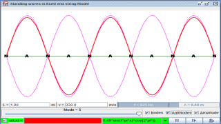
1) The “normal modes”, oscillatory patterns of definite frequency, are sine waves with a node at either end (and possibly other nodes in the middle). Specifically, the th normal mode is given by
2) The frequencies are given by
3) Since the system (in the ideal, low-amplitude case! – which is all you can solve easily without the computer) is perfecty linear, any number of normal modes, with any amplitudes, can coexist on the string without interfering. Any arbitrary excitation – like a plucked guitar string – is a superposition of many different normal modes with different amplitudes.
Let’s now see how well your string model reproduces these ideal properties.
-
Write initial-condition code to excite your string in any given normal mode with any given amplitude. Using a tension sufficient to stretch your string by at least twenty percent of its original length, try different normal modes at various amplitudes (ranging from “barely visible” to “large”). Does your model reproduce the expected qualitative behavior of the ideal vibrating string? In which regimes?
-
How does the behavior depend on the number of masses you have chosen? Should this affect the behavior at all? Is using a large more critical for modeling the low- normal modes, or the high ones? Why?
-
Now, write initial-condition code to excite your string with a Gaussian bump with any given width and location. Excite your string with narrow and wide Gaussians of modest amplitude, located both near the endpoints and near the center of the string. By observing the animation, comment on whether you have excited mostly the lower normal modes, or the higher ones.
-
If you have access to a stringed instrument (guitar, violin, ukelele, etc.), excite your real string in these ways (by plucking it with both your thumb and the edge of your fingernail, both near the center of the string and near the endpoint). How does the timbre of the sound produced correspond to the answers to your previous question?
Part 5: The low-amplitude limit, quantitatively
Now, let’s study the string’s vibrations precisely, and determine how well and under what conditions they align with the analytic predictions.
The quantitative thing that we can measure is the string’s period. To measure the period of any given normal mode , select a mass near an antinode of that mode, and watch it move up and down. If your initial conditions displace the string in the +y direction, then the string has completed one full period when the string moves “down, then back up, then starts to go down again”. To have our program tell us when that is, we want to watch for the time when the velocity changes from positive to negative.
In order to detect this, you’ll need to introduce a variable that keeps track of the previous value of at that position, so you can monitor it for sign changes.
- Modify your code to track the period, and measure the period of a normal mode of your choice. How does your result correspond to the analytic prediction in the low-amplitude regime for different normal modes? Vary the tension, mass, Young’s modulus, and length, and see if your simulation behaves as expected.
Part 6: Getting away from the low-amplitude limit
All of the things you’ve learned about the vibrating string – noninterfering superpositions of normal modes whose frequency is independent of amplitude – relate to solutions of the ideal wave equation. But deriving this equation from our model requires making the small-angle approximation to trigonometric functions, and this is only valid in the limit . Now it’s time to do something the pen-and-paper crowd can’t do (without a great deal of pain): get away from that limit.
- Try running your simulation at higher amplitudes using a variety of initial conditions. Play with this for a while. Do you still see well-defined normal modes with a constant frequency that “stay put”? Look carefully at the motion of each point; do they still move only up and down? Describe your observations.
Translations
| Code | Language | Translator | Run | |
|---|---|---|---|---|
 |
||||
Software Requirements
| Android | iOS | Windows | MacOS | |
| with best with | Chrome | Chrome | Chrome | Chrome |
| support full-screen? | Yes. Chrome/Opera No. Firefox/ Samsung Internet | Not yet | Yes | Yes |
| cannot work on | some mobile browser that don't understand JavaScript such as..... | cannot work on Internet Explorer 9 and below |
Credits

Fremont Teng; Loo Kang Wee; based on codes by W. Freeman
end faq
Version
- https://www.compadre.org/PICUP/exercises/exercise.cfm?I=151&A=vibrating-string
- http://weelookang.blogspot.com/2018/06/lattice-elasticity-vibrating-string-and.html
Other Resources
http://physics.bu.edu/~duffy/HTML5/transverse_standing_wave.html
