


About
Developed by E. Behringer
This set of exercises guides the student in exploring computationally the behavior of light patterns and shadows generated by simple light sources together with apertures in thin, opaque barriers. It requires the student to generate, and describe the results of simulating, light patterns and shadows. Diffraction is ignored. The numerical approach used is summing over a two-dimensional spatial grid while applying a logical mask (‘transparency function’). Please note that this set of computational exercises can be affordably coupled to simple experiments with small light bulbs and apertures cut into (or barriers cut out of) opaque paper sheets. A possible extension is to compare the predicted light patterns to experimental measurements. This set of exercises could be incorporated as an initial activity in an intermediate optics laboratory.
| Subject Area | Waves & Optics |
|---|---|
| Levels | First Year and Beyond the First Year |
| Available Implementation | Python |
| Learning Objectives |
Students who complete this set of exercises will be able to
|
| Time to Complete | 120 min |
EXERCISE 3: IRRADIANCE DUE TO POINT SOURCES AND AN L-SHAPED APERTURE
Now imagine that you have point sources, as in Exercise 2, but now the aperture is an L-shaped aperture as shown below.
What do you expect the irradiance pattern at the screen to look like? Why? Now calculate the irradiance pattern at the screen for the case and cm. Does the computed pattern resemble your prediction?
#
# Shadows_Exercise_3.py
#
# A linear array of N point sources located a specified distance from
# an L-shaped aperture composed of two rectangular apertures,
# one of which is centered on the origin.
# A screen is located a specified distance from
# the aperture.
#
# This file will generate a filled contour plot of
# the irradiance of light reaching the screen
# versus lateral coordinates (x,y)
#
# Written by:
#
# Ernest R. Behringer
# Department of Physics and Astronomy
# Eastern Michigan University
# Ypsilanti, MI 48197
# (734) 487-8799
# This email address is being protected from spambots. You need JavaScript enabled to view it.
#
# 20160112-13 by ERB one aperture
# 20160119 by ERB compound aperture
# 20160609 clean up by ERB
#
# import the commands needed to make the plot
from pylab import axis,xlim,ylim,xlabel,ylabel,show,contourf,colorbar,figure,title
from matplotlib import cm
# import the command needed to make a 1D array
from numpy import meshgrid,absolute,where,zeros,linspace
# inputs
zs = -20.0 # distance between the source and aperture [cm]
zsc = 40.0 # distance between the screen and aperture [cm]
nso = 101 # number of point sources
length_so = 4.0 # length of the array of point sources [cm]
ap1_width = 2.0 # aperture width [cm]
ap1_height = 1.0 # aperture height [cm]
ap2_width = 1.0 # second aperture width [cm]
ap2_height = 3.0 # second aperture height [cm]
ap2_x = -0.5 # second aperture center x-coordinate [cm]
ap2_y = 2.0 # second aperture center y coordinate [cm]
screen_width = 60.0 # screen width [cm]
screen_height = 60.0 # wcreen height [cm]
nw = 240 # Number of screen width intervals
nh = 240 # Number of screen height intervals
# initialize needed arrays to zero
rso = zeros((nso,2)) # (x,y) location of the source [cm,cm]
screen_x = zeros((nw+1,nh+1)) # x-coordinates of screen points
screen_y = zeros((nw+1,nh+1)) # y coordinates of screen points
rsq = zeros((nw+1,nh+1)) # r squared values
irradiance = zeros((nw+1,nh+1)) # irradiance values
x0 = zeros((nw+1,nh+1)) # x coordinate of intersection at aperture plane
y0 = zeros((nw+1,nh+1)) # y coordinate of intersection at aperture plane
# create 1D arrays to create a meshgrid for contour plotting
screen_xx = linspace(-0.5*screen_width,0.5*screen_width,nw+1)
screen_yy = linspace(-0.5*screen_height,0.5*screen_height,nh+1)
# generate the meshgrid
screen_xx, screen_yy = meshgrid(screen_xx,screen_yy)
# Set up point source coordinates
for i in range (0,nso):
for j in range (0,2):
if j==0: # the x-coordinate is
rso[i,j] = -0.5*length_so + i*length_so/(nso-1)
else: # j = 1 and the y-coordinate is
rso[i,j] = 0.0
# Calculate grid increments
deltaw = screen_width/nw # grid increment, width [cm]
deltah = screen_height/nh # grid increment, height [cm]
# Define the array of screen x and screen y values
for i in range (0,nw+1):
for j in range (0,nh+1):
screen_x[i,j] = -0.5*screen_width + deltaw*i
screen_y[i,j] = -0.5*screen_height + deltah*j
# Calculate the irradiance at each screen point
for k in range (0,nso):
for i in range (0,nw+1):
for j in range (0,nh+1):
# First calculate square of distance from source to screen
rsq[i,j] = (screen_x[i,j]-rso[k,0])**2 + (screen_y[i,j]-rso[k,1])**2 + (zsc-zs)**2
# Calculate x and y coordinates at the aperture
x0[i,j] = rso[k,0] + abs(zs)*(screen_x[i,j] - rso[k,0])/(zsc - zs)
y0[i,j] = rso[k,1] + abs(zs)*(screen_y[i,j] - rso[k,1])/(zsc - zs)
# Check if the ray coordinates at the aperture fall within the apertures
maskx1 = where(absolute(x0) < 0.5*ap1_width,1.0,0.0)
masky1 = where(absolute(y0) < 0.5*ap1_height,1.0,0.0)
maskx2 = where((x0 < ap2_x + 0.5*ap2_width)&(x0 > ap2_x - 0.5*ap2_width),1.0,0.0)
masky2 = where((y0 < ap2_y + 0.5*ap2_height)&(y0 > ap2_y - 0.5*ap2_height),1.0,0.0)
# Calculate the irradiance (note that we are accumulating irradiance)
irradiance = irradiance + (maskx1*masky1 + maskx2*masky2)/rsq
# make a filled contour plot of the period vs overlap and length ratios
figure()
contourf(screen_yy,screen_xx,irradiance,100,cmap=cm.bone)
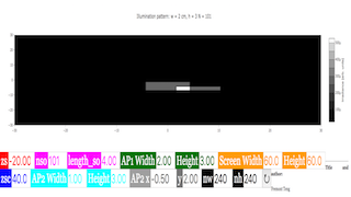
title('Illumination pattern: \(w = \)%s cm, \(h = \)%s; \(N = \)%d'%(ap1_width,ap1_height,nso))
axis('equal')
xlim(-0.5*screen_width,0.5*screen_width)
ylim(-0.5*screen_height,0.5*screen_height)
xlabel("\(x\) [cm]")
ylabel("\(y\) [cm]")
colorbar().set_label(label='Irradiance [arb. units]',size=16)
show()
Translations
| Code | Language | Translator | Run | |
|---|---|---|---|---|
 |
||||
Software Requirements
| Android | iOS | Windows | MacOS | |
| with best with | Chrome | Chrome | Chrome | Chrome |
| support full-screen? | Yes. Chrome/Opera No. Firefox/ Samsung Internet | Not yet | Yes | Yes |
| cannot work on | some mobile browser that don't understand JavaScript such as..... | cannot work on Internet Explorer 9 and below |
Credits

Fremont Teng; Loo Kang Wee
end faq
- https://www.compadre.org/PICUP/exercises/Exercise.cfm?A=Shadows&S=6
- http://weelookang.blogspot.com/2018/06/shadows-ray-optics.html