About

Subject Area	Electricity & Magnetism
Levels	First Year and Beyond the First Year
Available Implementation	Python
Learning Objectives	Students who complete this set of exercises will be able to: generate equations predicting the Cartesian components of force acting on the charged particle and generate the equations of motion for the particle (Exercise 1); calculate particle trajectories by solving the equations of motion (Exercise 2); produce two-dimensional and three-dimensional plots of the trajectories (Exercise 2); and simulate the operation of an E⃗ ×B⃗ $\overrightarrow{E}\times \overrightarrow{B}$ (Wien) filter (Exercise 3) and determine the range of particle velocities transmitted by the filter, and how these are affected by the geometry of the filter (Exercise 4).
Time to Complete	120 min

EXERCISE 3: THE E⃗ ×B⃗ $\overrightarrow{E}\times \overrightarrow{B}$ (WIEN) FILTER, PART 1

Regions of mutually perpendicular electric and magnetic fields can be used to filter a collection of moving charged particles according to their velocity. If we assume that a particle of velocity vpass=−Ey/Bx$v_{pass}=-E_y/B_x$ enters the field region traveling exactly along the z$z$-axis, the particle will experience zero net force and therefore zero acceleration and zero deflection from the z$z$-axis. If a small, circular aperture of radius R$R$ is placed on the z$z$-axis at z=L$z=L$, then this particle will be transmitted through the aperture.

(a) Use your program from Exercise 2 to determine the maximum value of vz,max=vpass+Δv$v_{z,max}=v_{pass}+\mathrm{\Delta }v$ for which an aperture of radius R=1.0$R=1.0$ mm will transmit the Li+${}^{+}$ ion (now assuming that vx=vy=0$v_x=v_y=0$). What is the value of Δv/vpass$\mathrm{\Delta }v/v_{pass}$?

(b) Repeat (a) for an aperture of radius R=2.0$R=2.0$ mm. What is the value of Δv/vpass$\mathrm{\Delta }v/v_{pass}$?

#

# ExB_Filter_Exercise_3.py

#

# This file is used to numerically integrate

# the second order linear differential equations

# that describe the trajectory of a charged particle through

# an E x B velocity filter.

#

# Here, it is assumed that the axis of the filter

# is aligned with the z-axis, that the magnetic field

# is along the +x-direction, and that the electric field

# is along the -y-direction.

#

# The numerical integration is done using the built-in

# routine odeint

#

# The specific goal of this code is to identify the

# maximumm value of v_z that permits transmission of the

# particles through the velocity filter with

# a specified exit aperture.

#

# By:

# Ernest R. Behringer

# Department of Physics and Astronomy

# Eastern Michigan University

# Ypsilanti, MI 48197

# (734) 487-8799 (Office)

# This email address is being protected from spambots. You need JavaScript enabled to view it.

#

# Last updated:

#

# 20160624 ERB

#

from pylab import figure,plot,xlim,xlabel,ylim,ylabel,grid,title,show,legend

from numpy import sqrt,array,arange,linspace,zeros,absolute

from scipy.integrate import odeint

#

# Initialize parameter values

#

q = 1.60e-19 # particle charge [C]

m = 7.0*1.67e-27 # particle mass [kg]

KE_eV = 100.0 # particle kinetic energy [eV]

Ex = 0.0 # Ex = electric field in the +x direction [N/C]

Ey = -105.0 # Ey = electric field in the +y direction [N/C]

Ez = 0.0 # Ez = electric field in the +z direction [N/C]

Bx = 0.002 # Bx = magnetic field in the +x direction [T]

By = 0.0 # By = magnetic field in the +x direction [T]

Bz = 0.0 # Bz = magnetic field in the +x direction [T]

R_mm = 1.0 # R = radius of the exit aperture [mm]

L = 0.25 # L = length of the crossed field region [mm]

u = [1.0,1.0,100.0]/sqrt(10002.0) # direction of the velocity vector

Ntraj = 1000 # number of trajectories

# Derived quantities

qoverm = q/m # charge to mass ratio [C/kg]

KE = KE_eV*1.602e-19 # particle kinetic energy [J]

R = 0.001*R_mm # radius of the exit aperture [m]

vmag = sqrt(2.0*KE/m) # particle velocity magnitude [m/s]

vzpass = -Ey/Bx # z-velocity for zero deflection [m/s]

# Set up the array of z-velocities to try

vz = vzpass + linspace(-0.25*vzpass,0.25*vzpass,Ntraj+1) # the set of initial z-velocities

particle_pass = zeros(Ntraj+1)

#

# Over what time interval do we integrate?

#

tmax = L/vzpass;

#

# Specify the time steps at which to report the numerical solution

#

t1 = 0.0 # initial time

t2 = tmax # final scaled time

N = 1000 # number of time steps

h = (t2-t1)/N # time step size

# The array of time values at which to store the solution

tpoints = arange(t1,t2,h)

#

# Here are the derivatives of position and velocity

def derivs(r,t):

# derivatives of position components

xp = r[1]

yp = r[3]

zp = r[5]

dx = xp

dy = yp

dz = zp

# derivatives of velocity components

ddx = qoverm*(Ex + yp*Bz - zp*By)

ddy = qoverm*(Ey + zp*Bx - xp*Bz)

ddz = qoverm*(Ez + xp*By - yp*Bx)

return array([dx,ddx,dy,ddy,dz,ddz],float)

# Specify initial conditions that don't change

x0 = 0.0 # initial x-coordinate of the charged particle [m]

dxdt0 = 0.0 # initial x-velocity of the charged particle [m/s]

y0 = 0.0 # initial y-coordinate of the charged particle [m]

dydt0 = 0.0 # initial y-velocity of the charged particle [m/s]

z0 = 0.0 # initial z-coordinate of the charged particle [m]

# Start the loop over the initial velocities

for i in range (0,Ntraj):

# Specify initial conditions

dzdt0 = vz[i] # initial z-velocity of the charged particle [m/s]

r0 = array([x0,dxdt0,y0,dydt0,z0,dzdt0],float)

# Calculate the numerical solution using odeint

r = odeint(derivs,r0,tpoints)

# Extract the 1D matrices of position values

position_x = r[:,0]

position_y = r[:,2]

# Check if the particle made it through the aperture

if absolute(position_x[N-1]) < R:

if absolute(position_y[N-1]) < sqrt(R*R - position_x[N-1]*position_x[N-1]):

particle_pass[i] = 1.0

else:

particle_pass[i] = 0.0

else:

particle_pass[i] = 0.0

# Look for the specific value of

for i in range (int(Ntraj/2),int(Ntraj)):#Frem:Added int

if absolute(particle_pass[i]-particle_pass[i-1]) > 0.5:

print("i = %d"%(i-1),"vz[i] = %.3e"%vz[i-1]," m/s.")#Frem:Added brackets

Deltav = vz[i-1] - vzpass

print("Delta v = %.3e"%Deltav," m/s.")#Frem:Added brackets

Deltavovervzpass = Deltav/vzpass

print("Delta v/vzpass = %.3e"%Deltavovervzpass)#Frem:Added brackets

# start a new figure

figure()

# Plot the particle pass function versus z-velocity

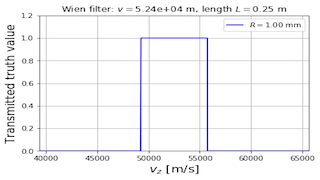
plot(vz,particle_pass,"b-",label='\(R = \)%.2f mm'%R_mm)

xlim(min(vz),max(vz))

ylim(0.0,1.2)

xlabel("\(v_z\) [m/s]",fontsize=16)

ylabel("Transmitted truth value",fontsize=16)

grid(True)

title('Wien filter: \(v = \)%.2e m, length \(L = \)%.2f m'%(vmag,L))

legend(loc=1)

show()

# start a new figure

figure()

# Plot the particle pass function versus scaled z-velocity

plot(vz/vzpass,particle_pass,"b-",label='\(R = \)%.2f mm'%R_mm)

xlim(min(vz/vzpass),max(vz/vzpass))

ylim(0.0,1.2)

xlabel("\(v_z/v_{z,pass}\)",fontsize=16)

ylabel("Transmitted truth value",fontsize=16)

grid(True)

legend(loc=1)

title('Wien filter: \(v_{z,pass} = \)%.2e m, length \(L = \)%.2f m'%(vzpass,L))

show()

 

Translations

Code	Language		Translator	Run

Software Requirements

	Android	iOS	Windows	MacOS
with best with	Chrome	Chrome	Chrome	Chrome
support full-screen?	Yes. Chrome/Opera No. Firefox/ Samsung Internet	Not yet	Yes	Yes
cannot work on	some mobile browser that don't understand JavaScript such as.....		cannot work on Internet Explorer 9 and below

 

Credits

Fremont Teng; Loo Kang Wee; based on codes by E. Behringer

end faq