
.png
)


About
Two dimensional vector fields
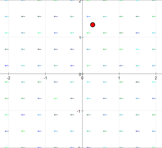
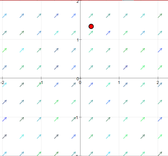
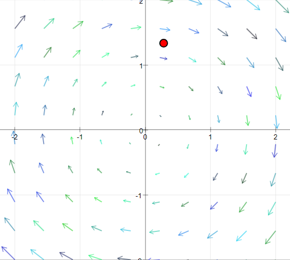
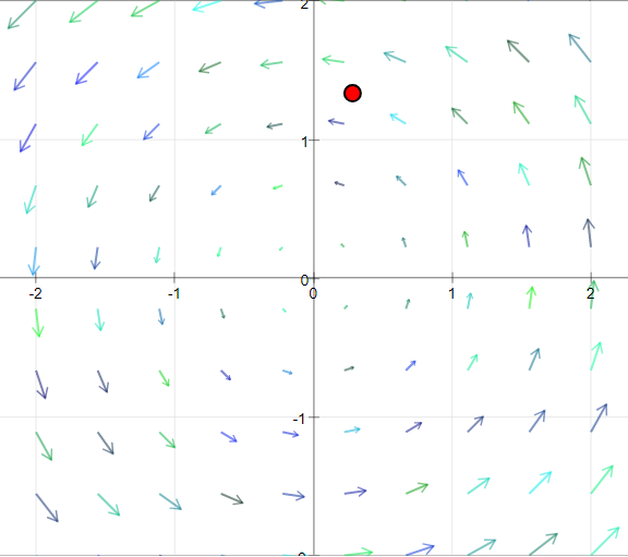
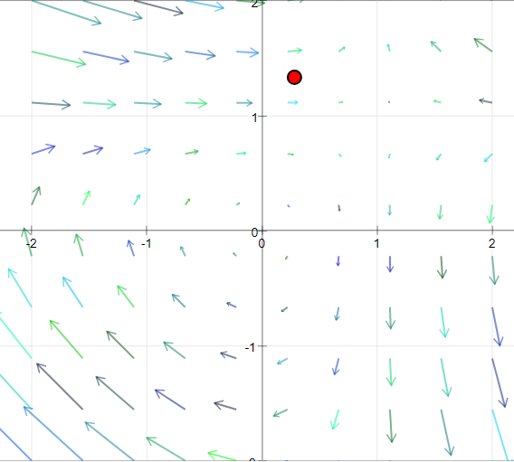
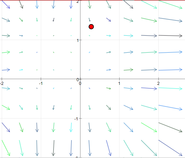
This simulation shows 2 dimensional vector fields, more specifically the xy cross section of a 3 dimensional vector field constant in z direction (as with a cylinder of infinite extension).
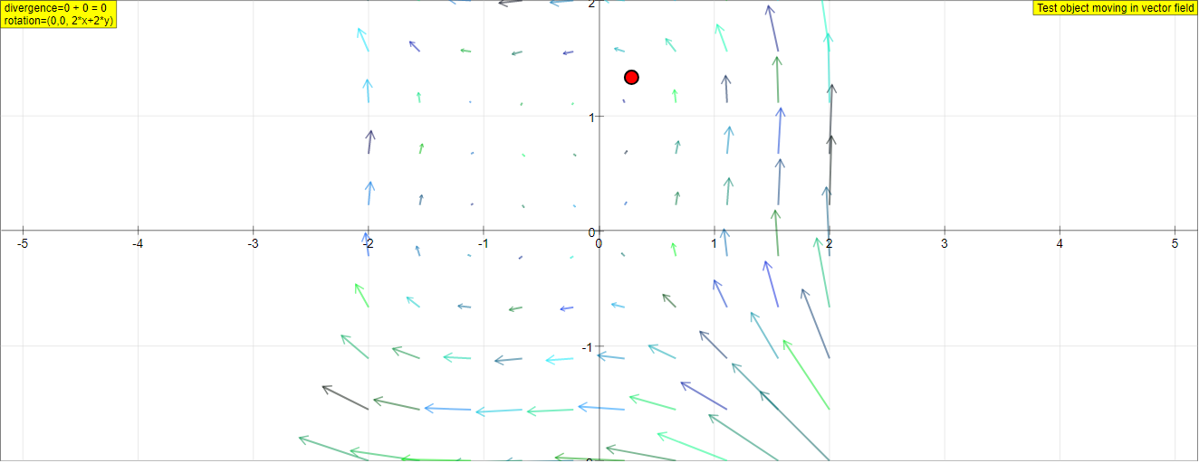
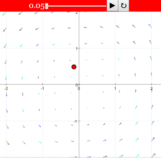
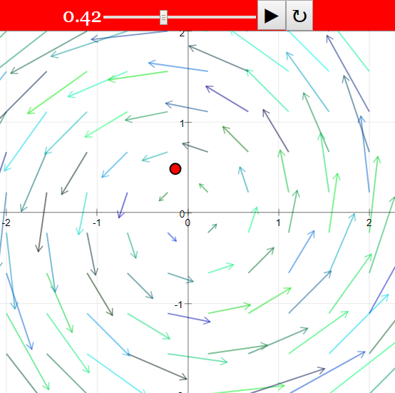
Shown are flow fields characterized by local velocity components a_x in the x direction and a_y in the y direction. Arrows with uniform length display the direction of the resulting flow vector. The size of the vector is indicated qualitatively by color gradation.
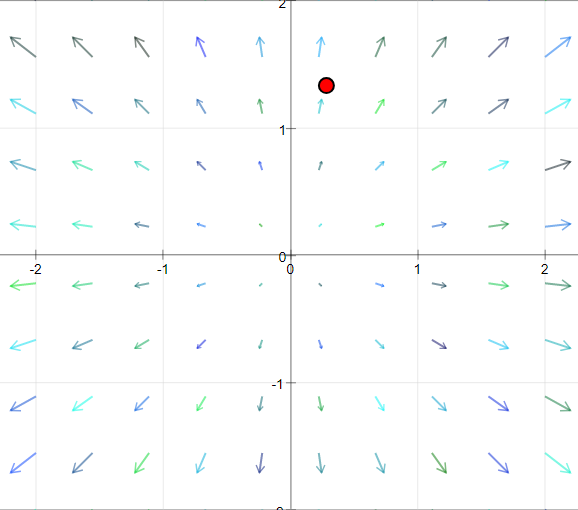
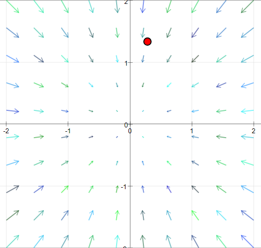
When opening the simulation, a field with two vortices is demonstrated. Two white text fields show the formulas of its vector components. A blue text field shows the divergence of the field, a brown field the 3D coordinates of its rotation vector.
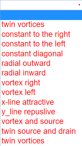
In a combobox one can choose among many predefined fields. The type of field and the components of its vectors are stated. The second case is empty for your own data insertions. Alternatively you can edit data of predefined cases in the a_x and a_y text fields (do not forget to press the Enter button after changes!)
Changing to another predefined function erases old data. If you want to preserve the result of your own changes, fabricate a picture, (most simply by pressing the Print button of your keyboard to transfer the window data into the temporary store; then paste them into a suitable document. A more comfortable way is to use a screenshot reader).
A red test object lies in the vector field that will follow the flow vector both in direction and value once the start button is activated. It jumps back to its initial position when it crosses the limits of the field. Step causes one step of movement.
You can draw the object with the mouse, and test the field at every position that way. This gives an impression of direction and value within the whole field.
You can turn off the vector arrows with an option switch and try to understand the field just from the movement of the test body.
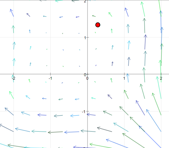
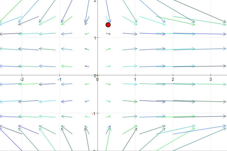
The zoom slider changes the scale of coordinates. As the number of arrows shown is constant, this helps to recognize details. The default case with two vortices is a good example.
The arrow length slider changes the length of arrows, init resets all parameters , reset_point resets the test object to the default position.
Vector Algebra
In this simulation the z component of the velocity vector is zero. The vector lies in the xy-plane. The rotation vector is perpendicular to the xy-plane; it has just a z component.
This results in:
a = (ax , ay, 0)
div a = ∂ax/∂x + ∂ay/∂y + 0 = ∂ax/∂x + ∂ay/∂y
rot v = (0, 0, ∂ay/∂x -∂ax/∂y)
When is the field without vortex: rotation = 0 ?
∂vy/∂x -∂vx/∂y = 0
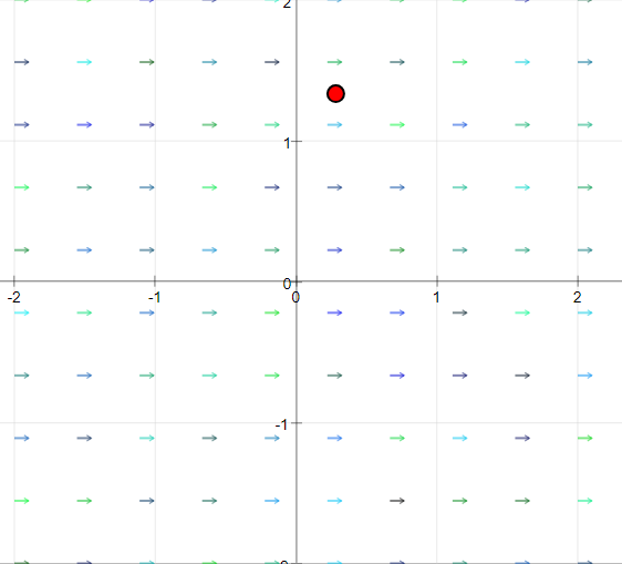
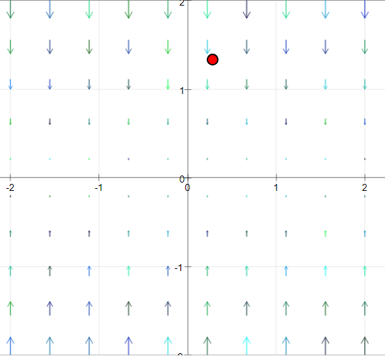
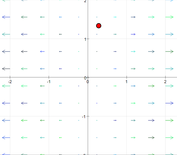
This holds when ax = a(x) and ay = a(y); the components are functions of their own coordinates only (e.g. ax = x2+3x-1, ay = y3-y2). This includes the case of both components being constants, whose derivative is zero (e.g. ax = 1, ay = -4).
If one component is a function of the other coordinate, then in general the field will have vortices, except when the partial derivatives just compensate, as for
rot (ax = y, ay = x) = (0, 0, 1 - 1) = (0, 0, 0 ) = 0
When is the field without source: divergence = 0?
∂ax/∂x = - ∂ay/∂y
The partial derivatives must be equal in absolute value, with opposite sign (sum = zero).
The movement of the test object is determined and calculated by two simple ordinary differential equations:
dx/dt = ax
dy/dt = ay
E 1: Study the default case of the twin vortices. Calculate rotation and divergence yourself by partial derivation of the formulas of the components (the "other" coordinate is treated as a constant).
E 2: Change the scale with the zoom slider and observe how the visual impression of the field changes with scale.
E 3: Start the test object and follow its path concerning direction and velocity. Try to understand this by studying the formulas.
E 4: Draw the test object to other points in the field and test its quantitative structure by the object´s movement.
E 5: Choose fields that have constants as components. Change numbers and understand how this influences the field. Start the test object. Does it change its velocity?
E 6: Choose fields with components linear in coordinates. Try to understand the context. Why are divergences not quoted? (localized limits may occur at sources).
E 6: How does the test object move now? Which terms in the formulas lead to acceleration?
E 7: Choose the two corresponding last cases of twin sources and twin vortices and study the differences.
E 8: Invent your own formulas for fields, calculate divergence and rotation, describe the characteristics.
Translations
| Code | Language | Translator | Run | |
|---|---|---|---|---|
 |
||||
Software Requirements
| Android | iOS | Windows | MacOS | |
| with best with | Chrome | Chrome | Chrome | Chrome |
| support full-screen? | Yes. Chrome/Opera No. Firefox/ Samsung Internet | Not yet | Yes | Yes |
| cannot work on | some mobile browser that don't understand JavaScript such as..... | cannot work on Internet Explorer 9 and below |
Credits
 Dieter Roess - WEH- Foundation; Fremont Teng; Loo Kang Wee
end faq
Sample Learning Goals
[text]
For Teachers
Two Dimensional Vector Fields JavaScript Simulation Applet HTML5
Instructions
Function Combo Box
Arrow Size Slider
Draggable Red Ball

Toggling Full Screen
Play/Pause and Reset Buttons

Research
[text]
Video
[text]
Version:
Other Resources
[text]