
.png
)


About
Riemann integral and Lebesgue integral
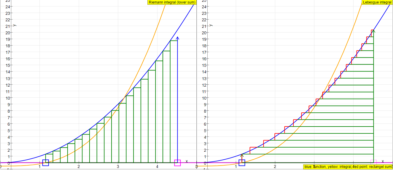
In two dimensions the Rieman integral determines the area between the x axis and the function y = f(x) by nesting it between two approximation sums. Both are constructed by a series of rectangles with intervals of the integration range along the x axis. For the upper sum the approximative value of y in each interval is equal to the largest value in the interval (its supremum); for the lower sum it is equal to the smallest value (infimum). The Riemann integral exists when both sums converge with decreasing interval width, and when they converge to the same limit. In this case it also exists for any value in the interval.
The Lebesgue întegral divides the integration area into stripes (not necessarily of the same width) parallel to the x axis (intervals along the y axis). The size of the area of each interval is characterized by a measure (taken parallel to the x axis), called the Lebesgue measure. If each stripe has a unique Lebesgue measure, the sum of the measures is the Lebesgue Integral.
The simulation uses as example a parabola y = x 2. The left window shows a Riemann infimum series, the right window a Lebesgue series, where the height of the first stripe is different from that of the other ones. The red line is the Lebesgue measure. It cuts the function at such a point that the area of the rectangle is equal to that of the stripe (which has a curved end in x direction). The spandrels to the left and to the right of the vertical red line have equal area.
The blue curve shows the parabola, whose antiderivative is to be calculated for an initial value x1 . The end point x2 of the integration range (magenta) can be drawn with the mouse. The yellow curve is the analytic solution y = (x 3 - x1 3) / 3.
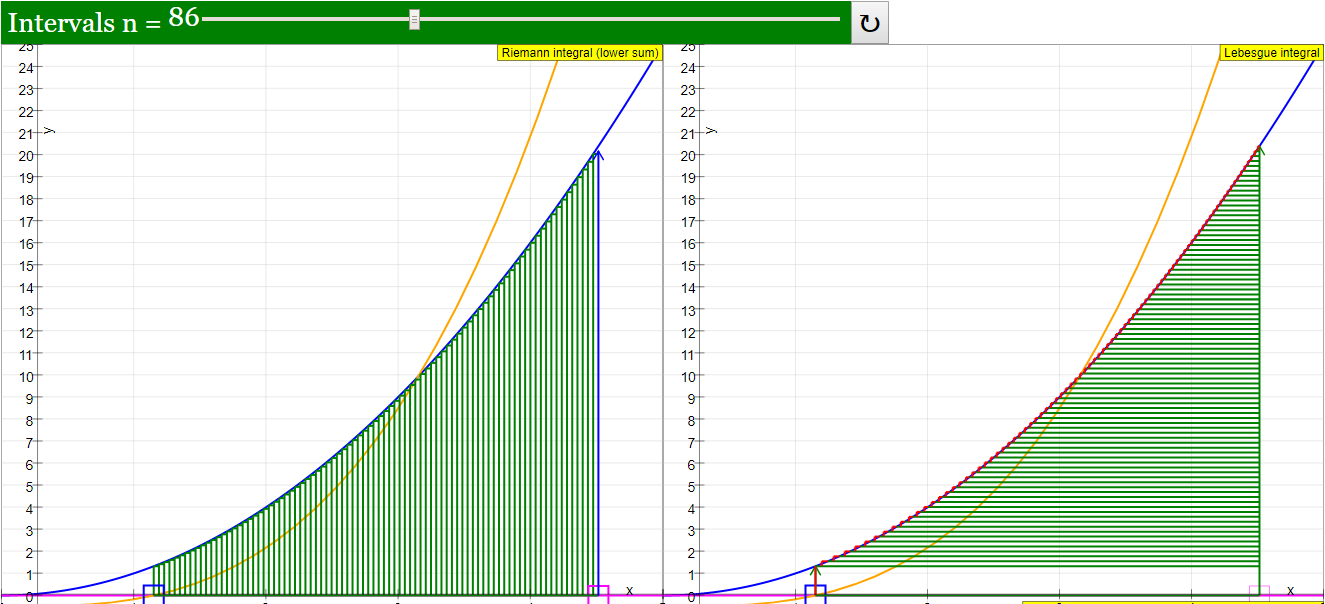
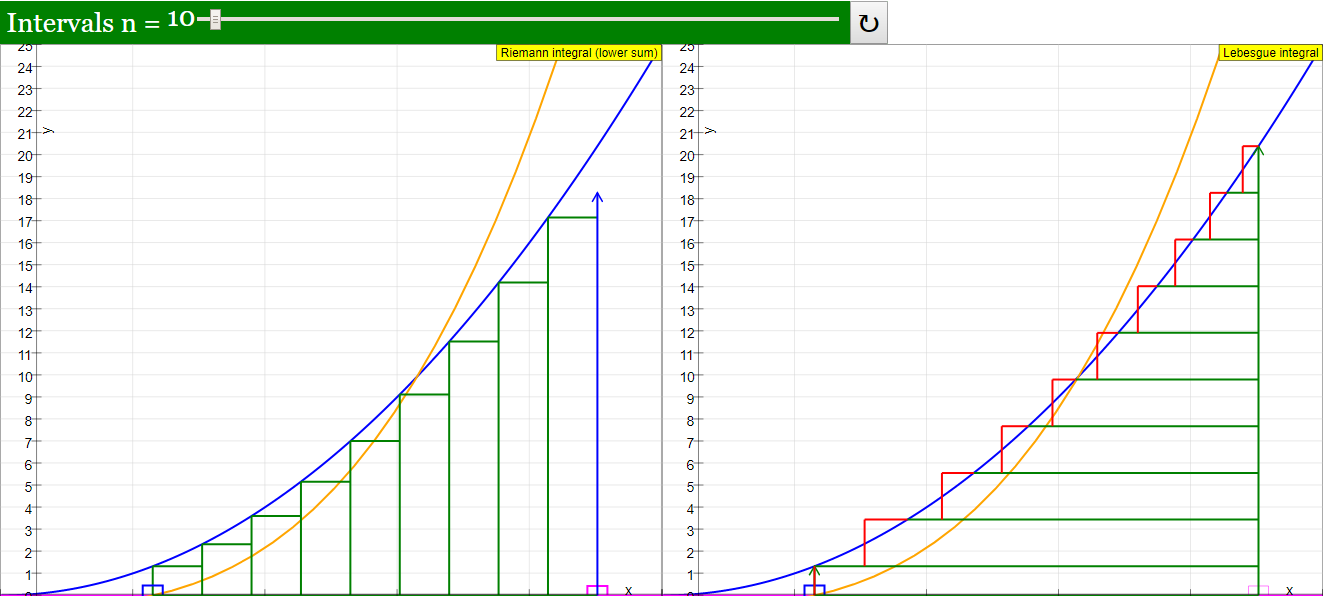
A first slider defines the initial point x1, a second slider the number of intervals n-1 (n in the Lebesgue case). Reset defines the integration range as 1 < x < 4 and n = 10.
In the Riemann construction the approximation gets better and better with increasing n. With the special definition of the Lebesgue measure chosen as an example, the coincidence is perfect independent of the number of intervals (the measure was calculated analytically; it could also be calculated in a limiting series process). The concept of the Lebesgue integral does not itself furnish a special method of calculation of its measures.
The strength of the Lebesgue concept lies in the very general mathematical applicability to the concept of integration. It can be applied to any set of objects, for which a measure is defined. A function that is Riemann integrable is always Lebesgue integrable, but not vice versa.
E1: Start with default settings: x1 = 1; x2 = 4; n = 10.
Verify that in the Riemann construction the intervals are closed by the infimum in the y-direction. Compare this to the Lebesgue construction. Consider the systematic deviations from the analytic value.
E2: Compare the Riemann lower sum construction with the numerical rectangle algorithm, starting at the initial point of the interval. Why are both identical in the parabola example, while they would be different for the sine function? (the parabola increases monotonically, while the sine oscillates).
E3: Increase the number of intervals and observe the Riemann lower sum approaching the analytic solution. What is the difference from the Lebesgue approximation (for the definition of the Lebesgue measure chosen in this example)?
Translations
| Code | Language | Translator | Run | |
|---|---|---|---|---|
 |
||||
Software Requirements
| Android | iOS | Windows | MacOS | |
| with best with | Chrome | Chrome | Chrome | Chrome |
| support full-screen? | Yes. Chrome/Opera No. Firefox/ Samsung Internet | Not yet | Yes | Yes |
| cannot work on | some mobile browser that don't understand JavaScript such as..... | cannot work on Internet Explorer 9 and below |
Credits
 Dieter Roess - WEH-Foundation; Fremont Teng; Loo Kang Wee
end faq
Sample Learning Goals
[text]
For Teachers
Riemann Integral and Lebesgue Integral JavaScript Simulation Applet HTML5
Instructions
n Slider
Draggable Boxes

Toggling Full Screen
Reset Button

Research
[text]
Video
[text]
Version:
Other Resources
[text]