
.png
)


About
"Derivative machine"
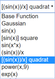
At the left side of the window one of 8 different predefined base functions y = f(x) can be selected by radio buttons. A suitable x range is attributed to each of them.
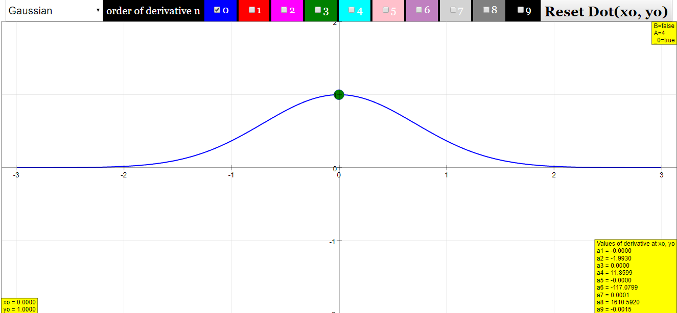
- Gaussian: exp (-(x-3)2)
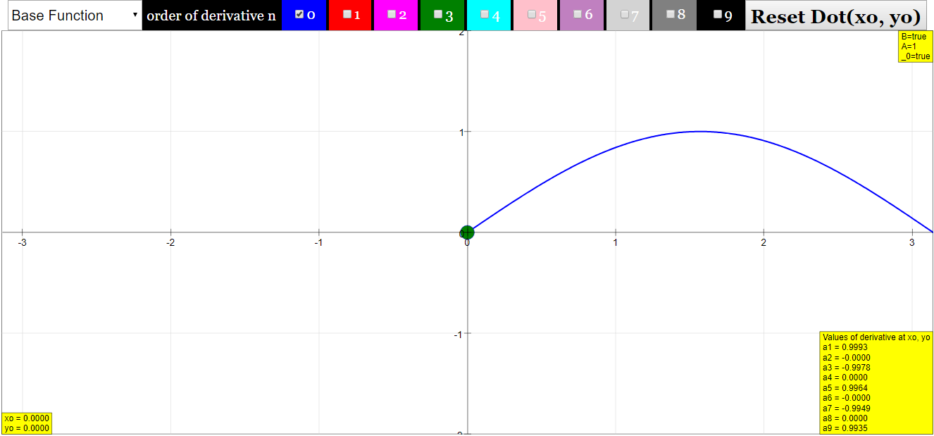
- sine (x)
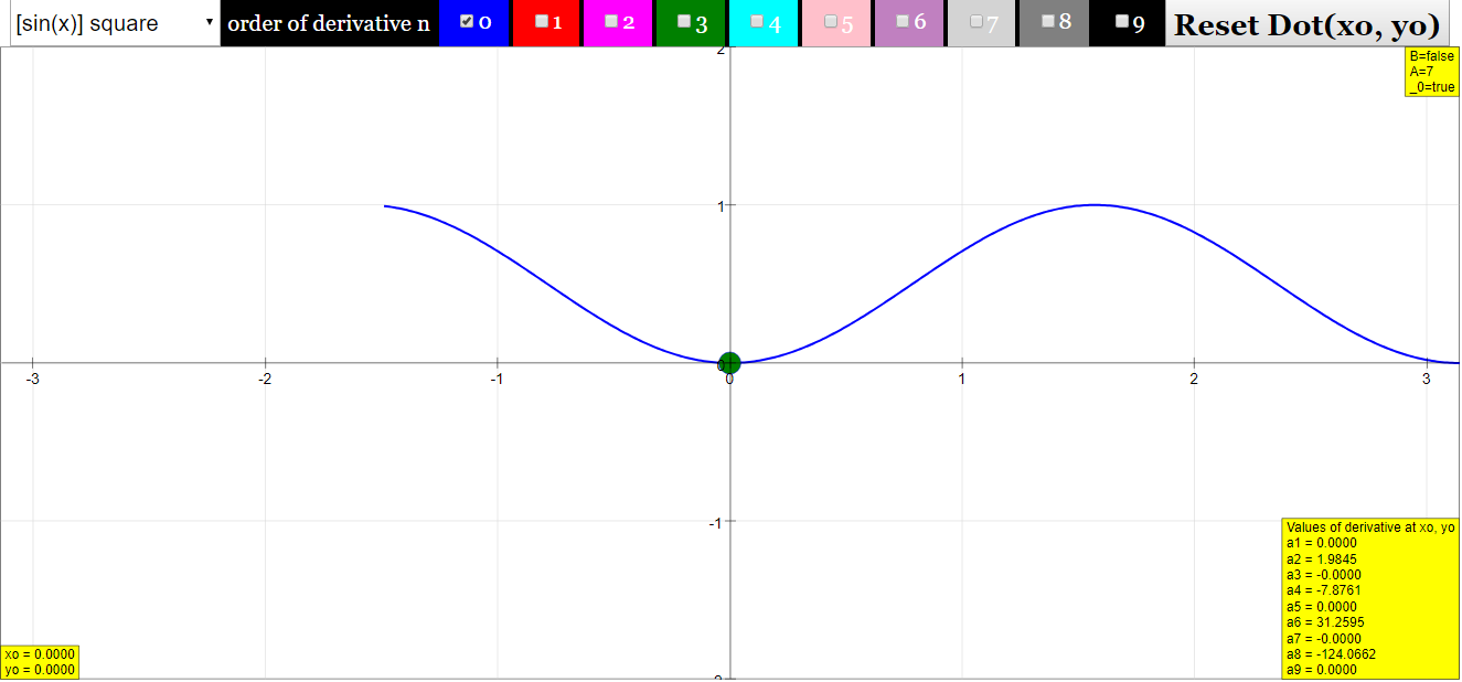
- (sine (x))2
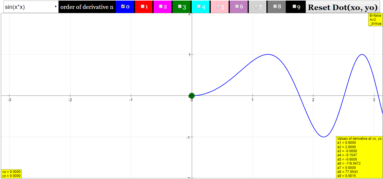
- sine (x2)
- (sine (x-20))/(x-20)
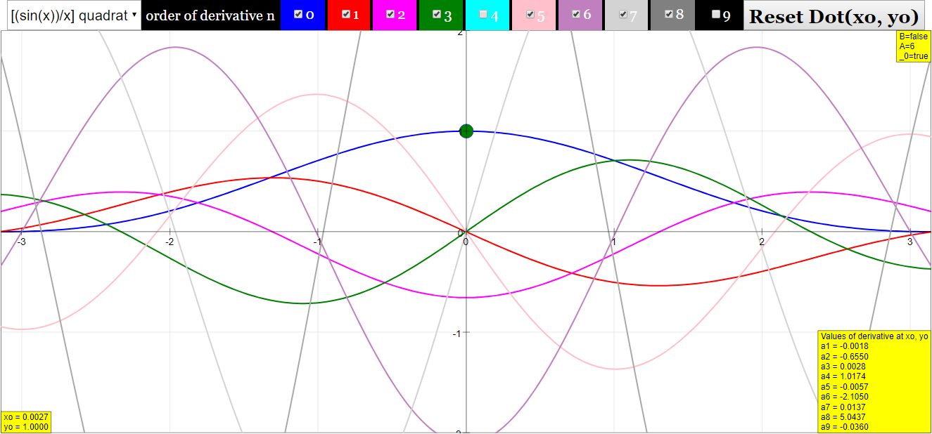
- [(sine (x-20))/(x-20)]2
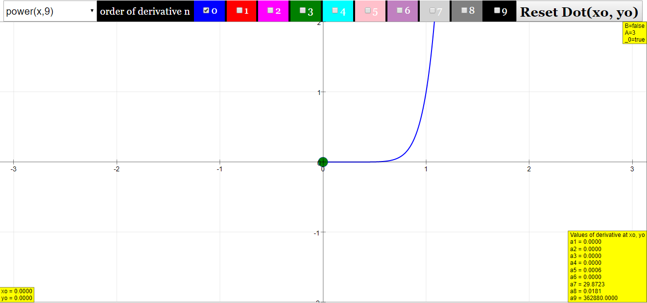
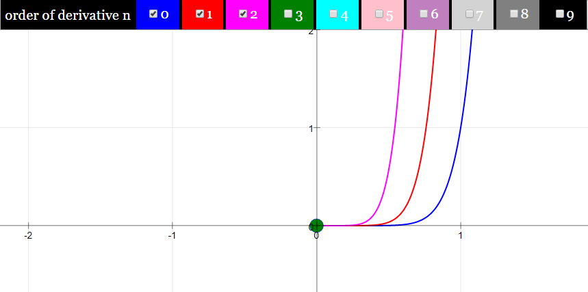
- Power function: pow (x,9) = x9 =x*x*x*x*x*x*x*x*x
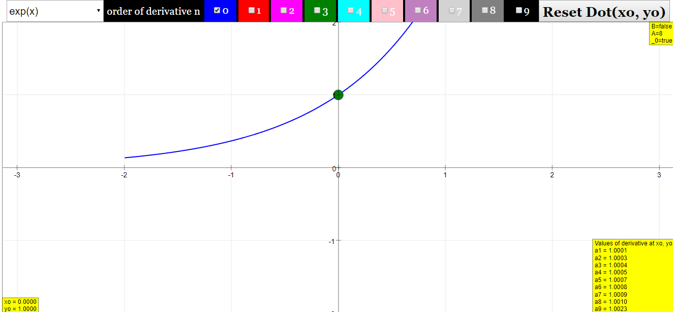
- Exponential: exp(x)
When the simulation is opened, the Gaussian function will be active. It is drawn as a blue curve. The zero line is shown in black.
At the top of the window there are 10 checkboxes to select derivatives of the base function. These are drawn as curves in the color of the check box numbers. Derivatives of different order can be shown simultaneously. Not all may be distinctly visible if their scales differ significantly. The scaling of the ordinate is self adjusting to the highest value.
A red dot on the curve defines a model point x0, y0 , for which the values of the derivatives a1 to a9 are shown in the number fields at the lower left. The dot can be drawn with the mouse to calculate derivatives for arbitrary model points. If it is drawn out of the abscissa range, it can be reset with the Reset Button.
Any one of the predefined functions can be selected with the Radio Buttons at the left.
For the sine function the curves of the 4th and the 8th derivative correctly coincide with that of the base function. The ninth derivative does not yet show visible irregularities by calculation or approximation errors.
With the power function, the 9th derivative is a very high constant. At high x values the limited resolution of the difference algorithm results in increasing noise-like deviations.
The functions in this simulation are not editable as in other simulations of this course. The reason is that this is the only way the results for high order derivatives can be calculated real time. If you want to investigate other functions, open the simulation with the EJS Console, and change or add the simple code for a predefined function.
Derivatives
This simulation calculates a base function
y = f(x)
for 1000 x- values in a given interval.
With h the difference between consecutive x values sufficiently small, the first derivative (differential quotient) is approximated by the difference quotient
y(1)(x) = (1/2h) [y(x+h) - y(x-h)]
The second derivative is approximated as the difference quotient of the first difference quotient
y(2)(x)= (1/2h) [y(1)(x+h) - y(1)(x-h)] = (1/2h)2 [y(x+2h) - 2y(x) + y(x-1h)]
This algorithm can be continued, leading to the code lines for the base function a[0] and the derivatives up to the 9th order a[9].
For the predefined functions and intervals most approximations do not visually differ from the analytical derivatives. This can be best controlled with the sine function, where the derivatives look the same at every 4th order.
For still higher derivatives, the limits of the accuracy of the approximation and also the computing accuracy are stressed, and noisy artifacts appear.
Code: With s = 1/(2h)
a0[j]=Math.pow(s,0)*y[0][j];
a1[j]=Math.pow(s,1)*(y2[1][j]-y1[1][j]);
a2[j]=Math.pow(s,2)*(y2[2][j]-2*y2[0][j]+y1[2][j]);
a3[j]=Math.pow(s,3)*(y2[3][j]-3*y2[1][j]+3*y1[1][j]-y1[3][j]);
a4[j]=Math.pow(s,4)*(y2[4][j]-4*y2[2][j]+6*y2[0][j]-4*y1[2][j]+y1[4][j]);
a5[j]=Math.pow(s,5)*(y2[5][j]-5*y2[3][j]+10*y2[1][j]-10*y1[1][j]+5*y1[3][j]-y1[5][j]);
a6[j]=Math.pow(s,6)*(y2[6][j]-6*y2[4][j]+15*y2[2][j]-20*y2[0][j]+15*y1[2][j]-6*y1[4][j]+y1[6][j]);
a7[j]=Math.pow(s,7)*(y2[7][j]-7*y2[5][j]+21*y2[3][j]-35*y2[1][j]+35*y1[1][j]-21*y1[3][j]+7*y1[5][j]-y1[7][j]);
a8[j]=Math.pow(s,8)*(y2[8][j]-8*y2[6][j]+28*y2[4][j]-56*y2[2][j]+70*y2[0][j]-56*y1[2][j]+28*y1[4][j]-8*y1[6][j]+y1[8][j]);
a9[j]=Math.pow(s,9)*(y2[9][j]-9*y2[7][j]+36*y2[5][j]-84*y2[3][j]+126*y2[1][j]-126*y1[1][j]+84*y1[3][j]-36*y1[5][j]+9*y1[7][j]-y1[9][j]);
The integers in the formulas follow simple generation rules, so that the series can be easily generated or continued.
E1:
- The first derivative describes the local steepness of the function´s curve
- The second derivative describes the local change of its steepness = curvature
- The third derivative describes the local change of its curvature = ?
- The fourth derivative describes the local change in the change of curvature or the curvature of the curvature of the base function = ??
- ...and so on
Try to understand what the higher derivatives mean, as applied to the base curve of a function
E2: Do the same for the sine function. Why does the 4th derivative look like the base function? (Hint: reason first why the second derivative looks like the negative of the base function, and then apply the same reasoning to the fourth and second derivative).
E3: Go through the derivatives of the power function: What type of parabola is each one?
(Hint: the easy way is to reason downward from the 9th one).
E4: Choose sine(x2). Consider why the derivatives assume higher and higher values (observe that the y scale is self adjusting!). Why are discernable oscillations shifting to higher x values with increasing order?
E5: With sine(x)/x many derivatives are within comparable amplitude range, while looking quite different. Go through exercise E1 to understand the change in the basic function expressed by the different derivatives.
(Hint: start by comparing any two consecutive derivatives)
Translations
| Code | Language | Translator | Run | |
|---|---|---|---|---|
 |
||||
Software Requirements
| Android | iOS | Windows | MacOS | |
| with best with | Chrome | Chrome | Chrome | Chrome |
| support full-screen? | Yes. Chrome/Opera No. Firefox/ Samsung Internet | Not yet | Yes | Yes |
| cannot work on | some mobile browser that don't understand JavaScript such as..... | cannot work on Internet Explorer 9 and below |
Credits
 Dieter Roess; Fremont Teng; Loo Kang Wee
Sample Learning Goals
[text]
For Teachers
Derivative Machine JavaScript Simulation Applet HTML5
Instructions
Function Box


Order of Derivatives Check Boxes
Reset Dot Button

Toggling Full Screen
Research
[text]
Video
[text]
Version:
Other Resources
[text]
end faq
{accordionfaq faqid=accordion4 faqclass="lightnessfaq defaulticon headerbackground headerborder contentbackground contentborder round5"}
- Details
- Written by Fremont
- Parent Category: Mathematics
- Category: Pure Mathematics
- Hits: 5690