
.png
)


About
Integral: algorithms of numerical approximation
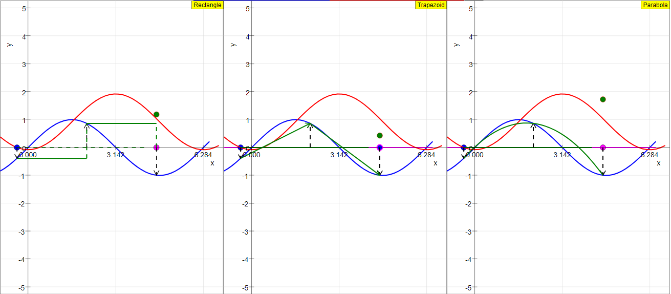
As an example for numerical integration we choose the sine function y = sin x ; its graph is shown in blue. The definite integral is to be calculated between an initial abscissa x1 and an end abscissa x2.
The analytic solution of the indefinite integral (antiderivative) is
y = ∫ sinxdx = -cos x +C
Its graph is shown in red, with C as the initial value at the initial abscissa.
The analytic definite integral is -(cos x2-cosx1). It corresponds to a point on the analytic curve at the end abscissa x2.
In the approximate numerical calculation the interval x2 - x1 is divided into n sub intervals of width delta. For clear demonstration of the principle n = 2 is chosen. Arrows show the value of the function in the three points of the double interval 2 delta.
Three numerical algorithms are visualized in three windows. They differ in how the approximative value of the function is defined between consecutive points in the sub interval delta.
1.) Rectangle approximation: y is taken as constant within the interval. The contribution of one interval is delta * y1.
2.) Trapezoid approximation: y is taken as the mean value within the interval. Its contribution is delta*(y1+y2)/2.
3.) Parabola approximation: the function in two consecutive intervals is approximated by a second order parabola through both end points and the middle point of the double interval (a parabola needs three points to be uniquely defined). The contribution of the double integral, derived as a surprisingly simple formula, is 2*delta*1/6(y1+4y2+y3).
In principle one can increase the precision of the parabola algorithm still further by using higher order parabolas, with correspondingly more sub intervals of the definition range. As the second order is already very good, higher order approximations have no great practical importance. (For fun and exercise derive the formula for a third order parabola!)
The simulation calculates the sum of two approximating intervals of width delta using the three algorithms. Their respective values are represented by the green points.
A first slider defines the interval delta, a second one the initial abscissa x1, reset defines delta = 1 and x1 = 0.5.
E1: Start with the default values : x1 = 0.5; delta=1
Compare how well the three procedures approximate the analytic solution.
E2: Draw the initial value with the mouse. Observe the shift of the analytic solution, and its relation to the result of the different algorithms. Explain mentally to some non professional what you observe!
E4: Reduce the interval width and observe how fast the approximations converge to the analytic solution.
E4: Keep the interval small and approximately constant while drawing the initial point. Observe whether the differences of the algorithms are comparable for all initial points. Interpret the result!
E5: For special initial points the simple algorithms result in exact agreement with the analytic value, while the parabola algorithms shows a recognizable deviation. Does this mean that the simple ones are better? What is the reason for identity in these cases?
Translations
| Code | Language | Translator | Run | |
|---|---|---|---|---|
 |
||||
Software Requirements
| Android | iOS | Windows | MacOS | |
| with best with | Chrome | Chrome | Chrome | Chrome |
| support full-screen? | Yes. Chrome/Opera No. Firefox/ Samsung Internet | Not yet | Yes | Yes |
| cannot work on | some mobile browser that don't understand JavaScript such as..... | cannot work on Internet Explorer 9 and below |
Credits

Dieter Roess - WEH-Foundation; Fremont Teng; Loo Kang Wee
Sample Learning Goals
[text]
For Teachers
Integral: Algorithms of Numerical Approximation JavaScript Simulation Applet HTML5
Instructions
Control Panel
Toggling Full Screen
Reset Button

Research
[text]
Video
[text]
Version:
Other Resources
[text]
end faq
{accordionfaq faqid=accordion4 faqclass="lightnessfaq defaulticon headerbackground headerborder contentbackground contentborder round5"}
- Details
- Written by Fremont
- Parent Category: Pure Mathematics
- Category: 5 Calculus
- Hits: 4414